Molecular Dynamics and Minimisation

OpenMM is an excellent package that provides a framework for running GPU-accelerated molecular dynamics (and related) simulations.

The Molecule, molecule view and container objects provide convenience functions that make it easier to use OpenMM to perform minimisation and molecular dynamics simulations.

Minimisation

You can perform minimisation on a molecule or collection of molecules using the minimisation() function. This returns a Minimisation object that can be used to control minimisation.

>>> import sire as sr
>>> mols = sr.load(sr.expand(sr.tutorial_url, "ala.top", "ala.crd"))
>>> mol = mols[0]
>>> print(mol.energy())
29.3786 kcal mol-1
>>> m = mol.minimisation()

You perform minimisation itself by calling the run() function.

>>> m.run()
minimisation ✔
Minimisation()

You can extract the results of minimisation, converted back into the original view object by calling commit()

>>> mol = m.commit()
>>> print(mol.energy())
17.7799 kcal mol-1

You could run all of these steps on a single line, e.g.

>>> mol = mols[0].minimisation().run().commit()
>>> print(mol.energy())
minimisation ✔
17.7799 kcal mol-1

In the above case we minimised just the first molecule that was loaded. We can minimise all molecules by calling minimisation on the whole collection.

>>> print(mols.energy())
-5855.24 kcal mol-1
>>> mols = mols.minimisation().run().commit()
>>> print(mols.energy())
minimisation ✔
-7971.79 kcal mol-1

Molecular Dynamics

You can perform molecular dynamics on a molecule or collection of molecules using the dynamics() function. This returns a Dynamics object that can be used to control dynamics.

>>> import sire as sr
>>> mols = sr.load(sr.expand(sr.tutorial_url, "ala.top", "ala.crd"))
>>> mol = mols[0]
>>> d = mol.dynamics()

You run dynamics by calling the run() function. You pass in the amount of time you want to simulate, and (optionally) the amount of time between saved coordinate/velocity snapshots.

For example, here we will run 10 picoseconds of dynamics, saving a frame every 0.5 picoseconds

>>> d.run(10*sr.units.picosecond, 0.5*sr.units.picosecond)
Dynamics(completed=10 ps, energy=-8.82722 kcal mol-1, speed=119.2 ns day-1)

Note

The speed of the simulation will depend on whether or not you have a GPU, and how fast it is. Reduce the simulation time if you find the above example takes too long.

You can extract the results of dynamics by calling commit().

>>> mol = d.commit()
>>> mol.view()

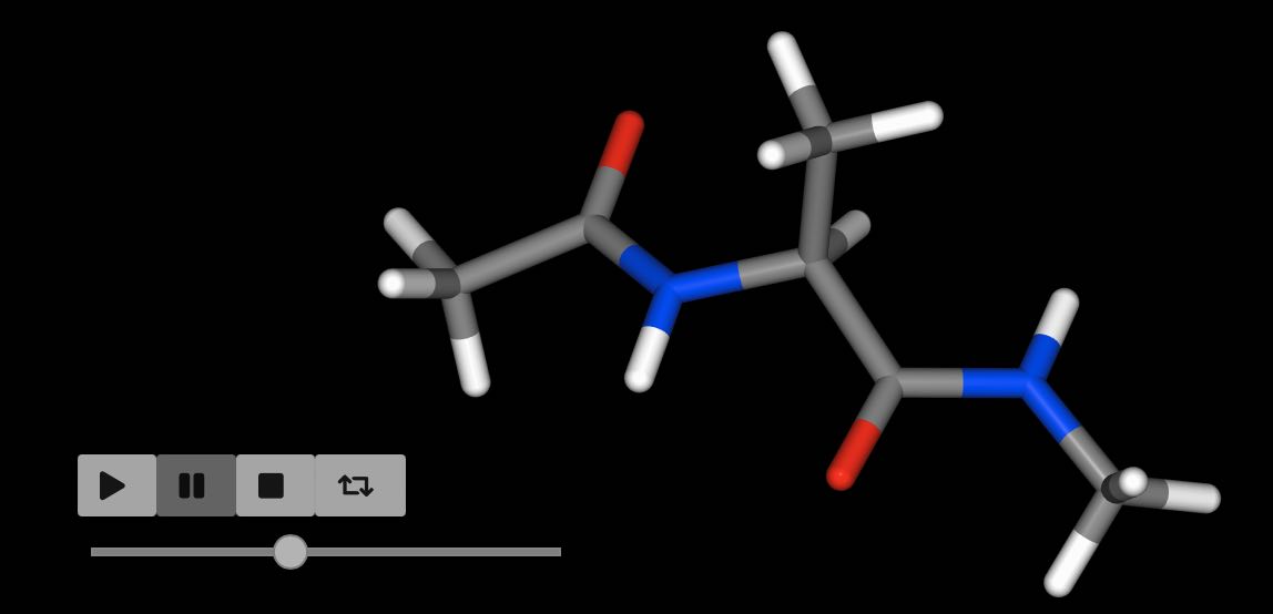
In this case, we performed molecular dynamics on just the first molecule of the loaded system. We can perform dynamics on all the molecules by calling dynamics() on the complete collection.

>>> d = mols.dynamics()
>>> d.run(10*sr.units.picosecond, 0.5*sr.units.picosecond)
Dynamics(completed=6010 ps, energy=-5974.09 kcal mol-1, speed=80.5 ns day-1)
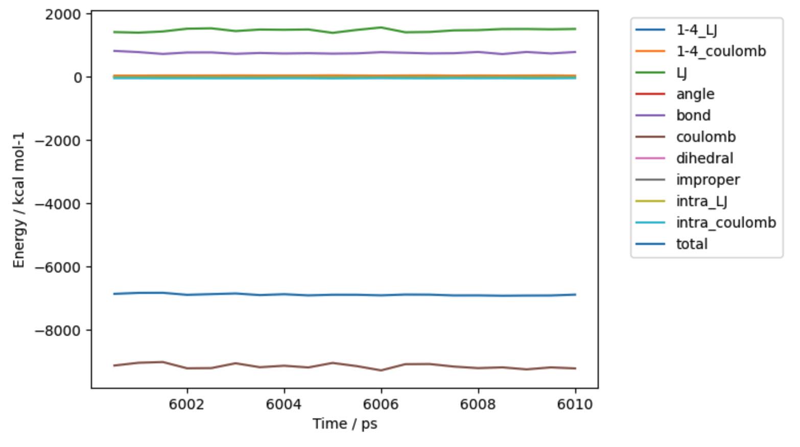
>>> mols = d.commit()
>>> mols.trajectory().energy().pretty_plot()

Note

The input file was the end-point of 6 ns of dynamics. We’ve now just run an additional 10 ps of dynamics, hence why it list that 6010 ps have been completed.

The frames from dynamics are stored as a trajectory in the molecules. They can be processed using the trajectory functions introduced previously. In this case we called pretty_plot on the energy to get a nice graph of the component energies versus time.

You can continue running more dynamics by calling the run() function again. You can choose different intervals to save frames for each run. For example, you could have a long “equilibration” run that doesn’t save frames at all by setting save_frequency to 0.

>>> d.run(10*sr.units.picosecond, save_frequency=0)
Dynamics(completed=6020 ps, energy=-5974.9 kcal mol-1, speed=89.2 ns day-1)

You can run as many blocks as you like, e.g.

>>> d.run(1*sr.units.picosecond, save_frequency=0.01*sr.units.picosecond)
Dynamics(completed=6021 ps, energy=-5974.61 kcal mol-1, speed=84.4 ns day-1)
>>> d.run(50*sr.units.picosecond, save_frequency=1*sr.units.picosecond)
Dynamics(completed=6071 ps, energy=-5976.05 kcal mol-1, speed=58.3 ns day-1)
>>> mols = d.commit()
>>> mols.view()

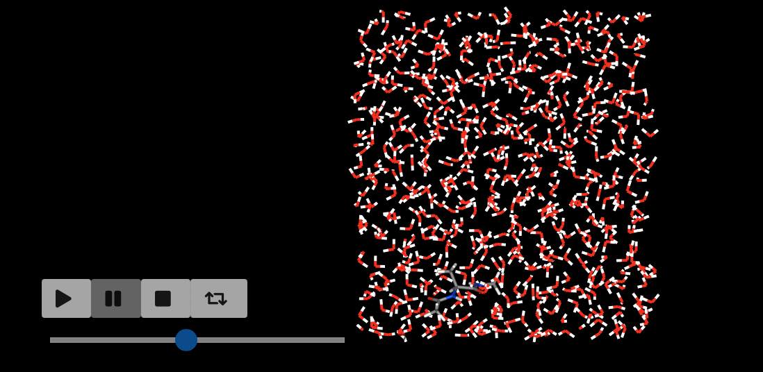
When you play the movie of the trajectory you should see the slow-motion section when 100 frames were saved over a 1 ps period, and then the fast-motion when 50 frames were saved over a 50 ps period.

Controlling Dynamics

There are several parameters that are needed to control the molecular dynamics simulation. By default, sire will do a good job trying to guess them based on what it can find in the molecules being simulated.

You can manually override this choice via a number of methods.

The easiest is to pass additional options to the dynamics() function when you first create the Dynamics object. Available options are;

• cutoff - set the cutoff distance for non-bonded interactions. By default this is 7.5 Å.

• cutoff_type - set the method used for the non-bonded cutoff. By default this is particle mesh Ewald (PME).

• timestep - set the timestep used for the integrator. By default this is 1 femtosecond (fs).

• save_frequency - the default value of save_frequency if this is not specified in run(). By default this is 25 picoseconds (ps).

• constraint - the level of constraints to apply to the molecules, e.g. constraining bonds, angles etc. By default this is inferred from the value of timestep. It defaults to no constraints. But timesteps greater than 1 femtoseconds will constrain all bonds involving hydrogen and all angles involving hydrogen. Timesteps greater than 2 femtoseconds will constrain all bonds, and all angles involving hydrogen.

For example

>>> d = mols.dynamics(cutoff_type="reaction_field",
...                   timestep=4*sr.units.femtosecond,
...                   save_frequency=1*sr.units.picosecond)
>>> d.run(10*sr.units.picosecond)
Dynamics(completed=6081 ps, energy=-6601.59 kcal mol-1, speed=432.2 ns day-1)

will perform 10 picoseconds of dynamics saving a frame every 1 picosecond. The reaction field cutoff scheme will be used, with an integration timestep of 4 femtoseconds. Since a larger timestep was used, constraints were automatically applied to all bonds, and all angles involving hydrogen. This simpler cutoff scheme plus larger timestep has lead to a much faster simulation (in this case, >400 nanoseconds per day, compared to ~60-80 nanoseconds per day above).

Another way to pass in options is to use the map option. This lets you pass in a dictionary of key-value pairs that provide extra configuration options for the Dynamics object.

This can be useful as a way of creating a dictionary of parameters that can be re-used between multiple dynamics runs.

>>> m = {"cutoff_type": "reaction_field",
...      "timestep": 4*sr.units.femtosecond,
...      "save_frequency": 1*sr.units.picosecond}
>>> d = mols.dynamics(map=m)
>>> d.run(10*sr.units.picosecond)
Dynamics(completed=6081 ps, energy=-6601.01 kcal mol-1, speed=439.8 ns day-1)
>>> d2 = mols.dynamics(map=m)
>>> d2.run(10*sr.units.picosecond)
Dynamics(completed=6081 ps, energy=-6601.01 kcal mol-1, speed=440.6 ns day-1)

The parameter map approach can be used to set other properties of the simulation. More details on what properties can be set, and how to query the value of set properties can be found here.