Viewing Molecules

sire has integrations with NGLView and RDKit to enable you to easily create two dimensional and three dimensional views of molecules. These are available via the view2d() and view() functions that are available for every molecule, molecule view, collection and system object. Calling view2d() or view() will view whatever molecular data is contained within that object in either 2D or 3D.

2D Views

Creating 2D structure views is very straightforward. Simply call the view2d() member function of the object that contains the molecular data you want to view.

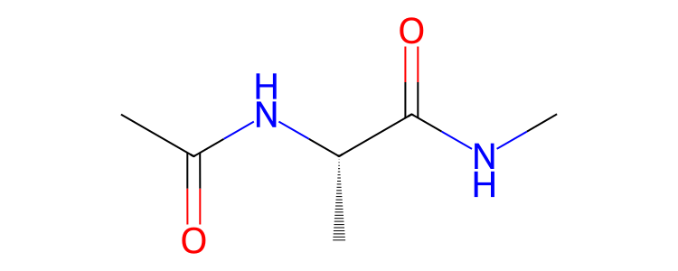
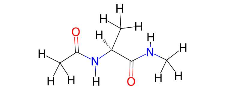
For example, (in a Jupyter notebook or similar) you can view individual molecules…

>>> import sire as sr
>>> mols = sr.load(sr.expand(sr.tutorial_url, "ala.top", "ala.crd"))
>>> mol = mols[0]
>>> mol.view2d()

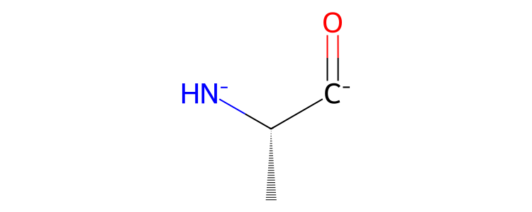
or parts of molecules.

>>> res = mol["residx 1"]
>>> res.view2d()

Note

Note that the charge and bond state of partial molecules may be incorrect. This is because the algorithm that assigns charges and bonds will see that the atoms whose bonds have been broken are missing electrons in their valence shell. The algorithm will try to correct this by adding or removing extra bonds, or adding or removing electrons from those atoms.

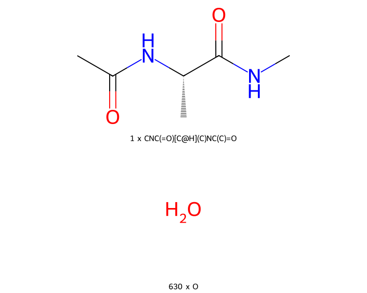
You can even view collections of molecules. In this case, molecules are grouped together by structure, and you see the number of each type of molecules in the collection.

>>> mols.view2d()

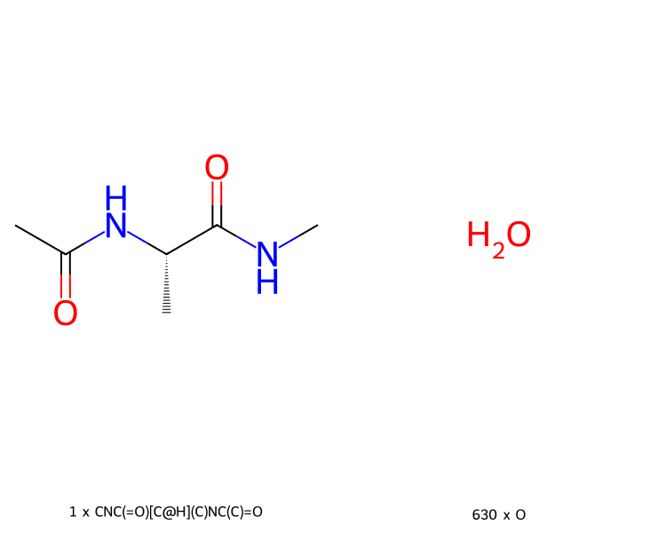
By default, the molecules are printed in a single column. You can print the molecules across multiple columns by setting their number via the num_columns argument, e.g.

>>> mols.view2d(num_columns=2)

If you aren’t working in a Jupyter notebook (or similar), or if you want to save the images to a file, simply pass your desired filename as the filename argument, e.g.

>>> mols.view2d(filename="structure.png")
/path/to/structure.png'

This returns the full path to the image that was created. The image format will be chosen based on the file extension. Supported formats are SVG (.svg), PNG (.png) and PDF (.pdf). Note that you may need to install the cairosvg library to save to PNG or PDF. If you don’t have this installed, then a warning will be printed and the image will be saved in SVG format (with the file extension changed to .svg).

By default, the image size for both displaying in a notebook and saving to a file is 750x300 pixels for single-molecule views, and 750x600 pixels for multi-molecule views. You can control the image size via the height and width options, e.g.

>>> mols.view2d(filename="structure.png", height=1000, width=1000)
/path/to/structure.png'

Also, by default, this structure view will only include hydrogens where they are needed to resolve any ambiguities. Unambiguous hydrogens are not shown. You can view them by passing include_hydrogens==True, e.g.

>>> mol.view2d(include_hydrogens=True)

The bond state (single, double, aromatic etc.), formal charge and stereochemistry of the atoms and bonds in the molecule(s) is determined automatically if this information is not present within the molecule(s)’s properties. A simple, yet effective algorithm described here has been copied into sire. This algorithm loops over atoms and adds or removes bonds and electrons such until each atom has filled its valence shell. The stereochemistry is determined using the AssignStereochemistryFrom3D function from RDKit, based on the coordinates in the coordinates property. As with all of sire, you can change the properties used to find information from a molecule by passing in a property map via the map argument of view2d().

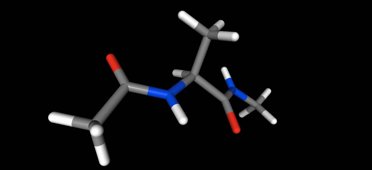
3D Views

Creating 3D views is similarly straightforward. Simply call the view() function on the object that contains the molecule data you want to view. This will start an interactive 3D viewer that you can use to rotate, translate and zoom around. If the molecule has multiple trajectory frames, then you will also get video player controls to play, pause, stop and scroll through an animation of each frame.

Note

3D views can only be created within Jupyter notebooks (or similar). There is no option currently to let you save the image to a file.

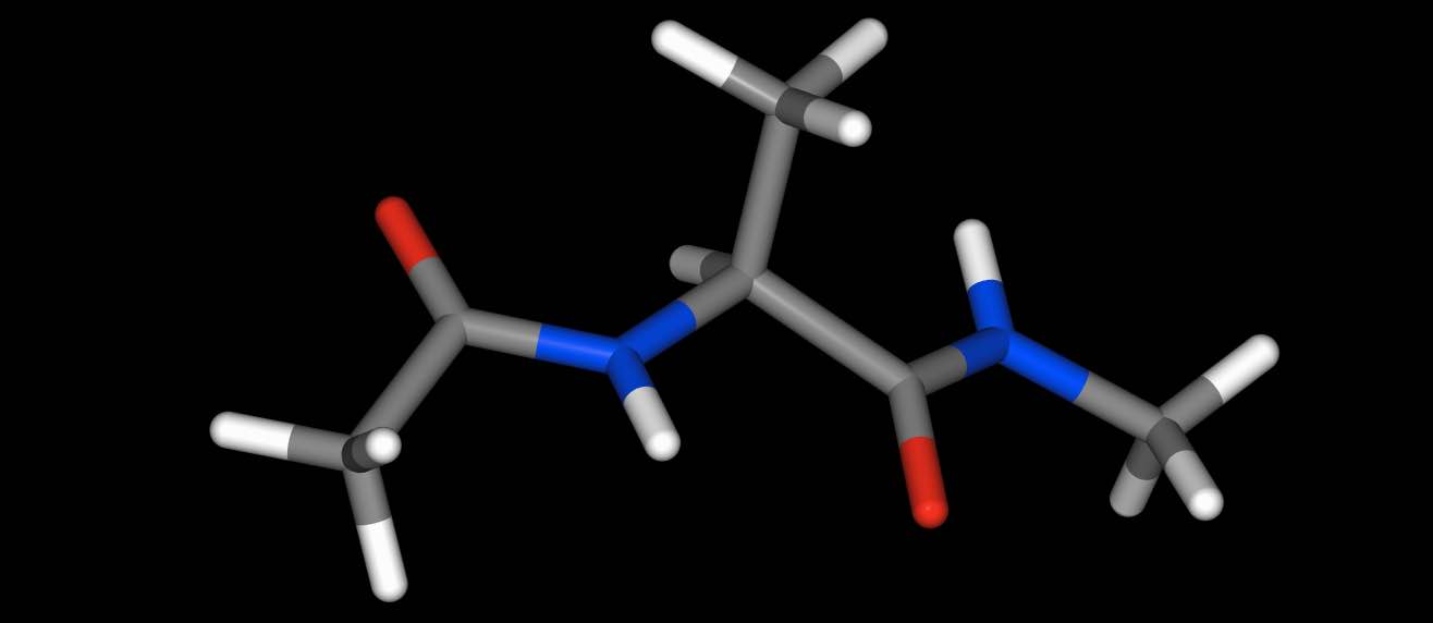
You can view individual molecules…

>>> import sire as sr
>>> mols = sr.load(sr.expand(sr.tutorial_url, "ala.top", "ala.crd"))
>>> mol = mols[0]
>>> mol.view()

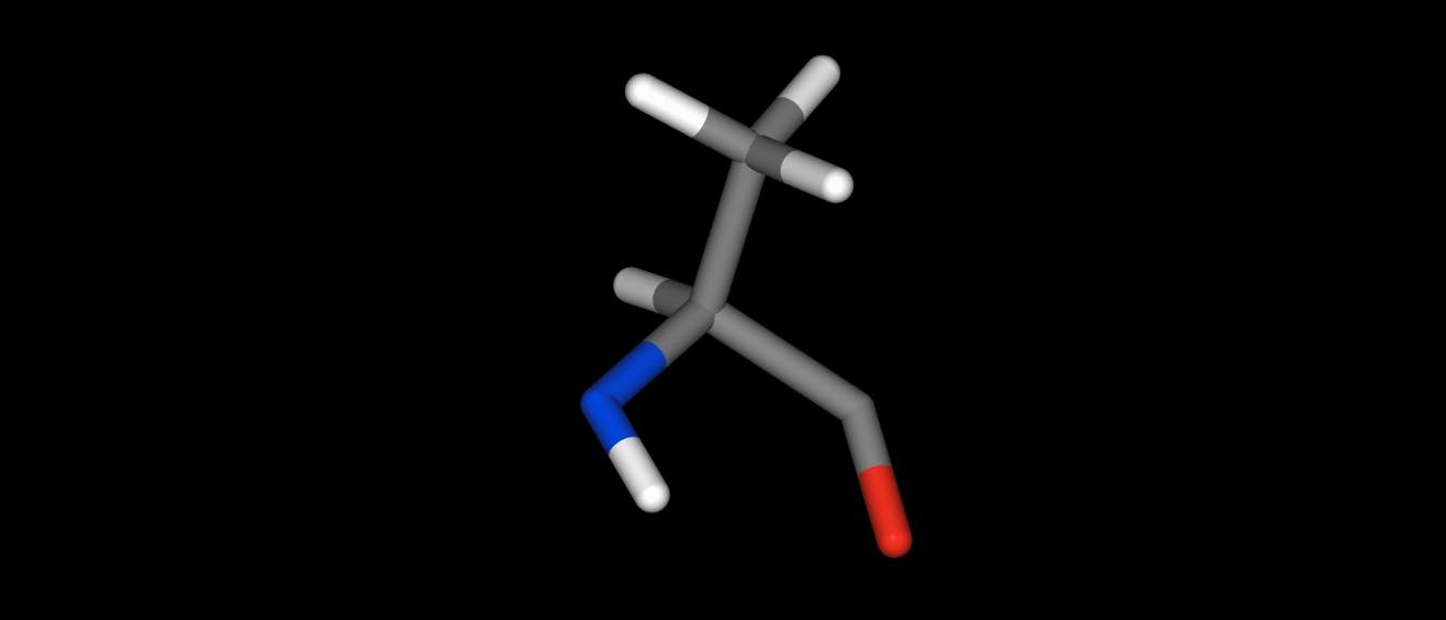
parts of molecules…

>>> res = mol["residx 1"]
>>> res.view()

or even whole collections of molecules.

>>> mols.view()

By default, the 3D view is orthographic. You can switch to a perspective view by passing orthographic=False, e.g.

>>> mol.view(orthographic=False)

Choosing the 3D representation

You can control the representation used for the view via the additional arguments of the function.

• protein - set the representation used for protein molecules

• water - set the representation used for water molecules

• ion - set the representation used for single-atom ions

• default or rest - set the representation used for all other molecules (e.g. ligands)

You can also force all molecules to use the same representation by setting the all option.

Setting any of the above to None, False or the string none will switch off that view. Setting default to None or False, or setting no_default to True will disable all default views.

NGLView provides several representations that you can use. These are:

• ball_and_stick - a ball and stick view

• base - simplified DNA/RNA base view

• cartoon - traditional “cartoon” view of a protein

• hyperball - smoothly-connected ball and stick view

• licorice - prettier line view

• line - simple line view

• point - simple point for each atom

• ribbon - show the protein backbone as a ribbon

• rocket - rocket view

• rope - show the backbone as a rope

• spacefill - Spacefilled spheres for each atom

• surface - Render the molecular surface only

• trace - trace view

• tube - show the backbone as a rope

So setting protein="tube" would render protein molecules with a tube representation. Setting all="spacefill" would render all atoms using a spacefill representation etc.

The following default representations will be used:

• protein - cartoon:sstruc

• water - line:0.5

• ion - spacefill

• default - hyperball

Note

The sstruc and 0.5 values refer to colors, which are described in the next section.

Note

We use default to refer to any other molecule, e.g. typically ligands.

You can switch off the default representations by passing no_default=True, e.g. mols.view(no_default=True, protein="surface") would show only the surface view of a protein. You can also switch off all default representations by passing default=False, default=None, all=False or all=None.

You can also pass multiple representations per view by passing in a list of representations, e.g.

>>> mols = sr.load("3NSS")
>>> mols.view(protein=["tube", "licorice"])

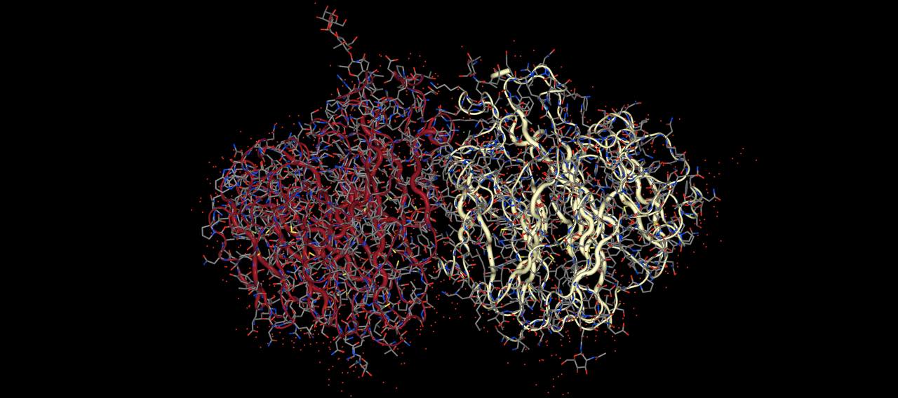
views the protein with both a licorice and a tube representation.

The terms protein, water and ion are performing searches of the molecule(s) for all atoms that match those search terms. You can create your own selections by passing in search terms for arguments that match the representation. For example

>>> mols.view(spacefill="resname ALA")

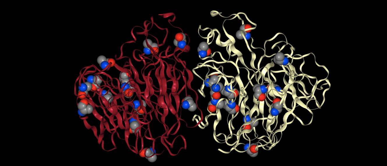
will render the protein in default view (cartoon) and will additionally render every atom that matches resname ALA in spacefill.

You can match multiple search terms by passing them in as a list, e.g. mols.view(spacefill=["resname ALA", "resname ASP"]) would render both ALA and ASP residues in spacefill.

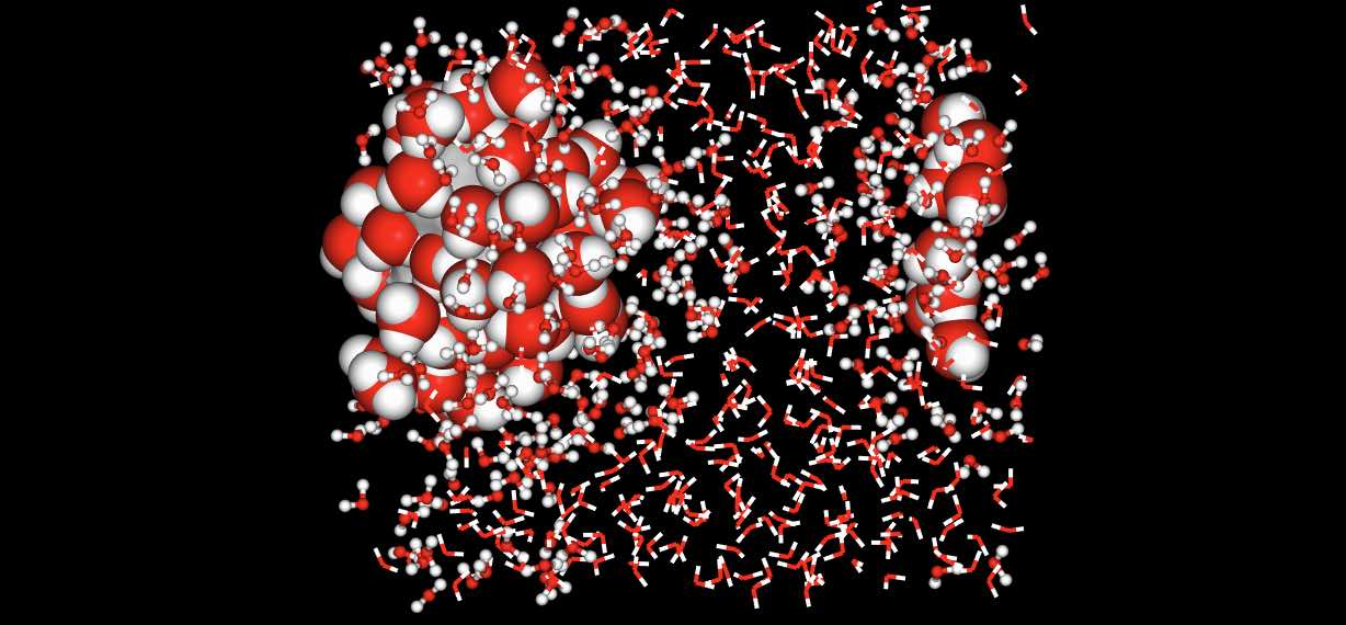
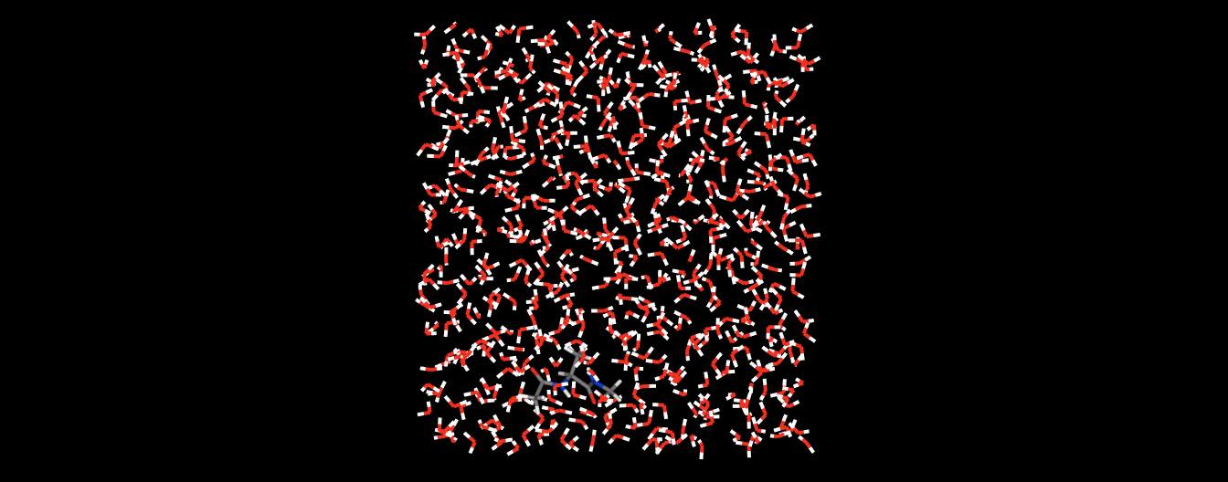
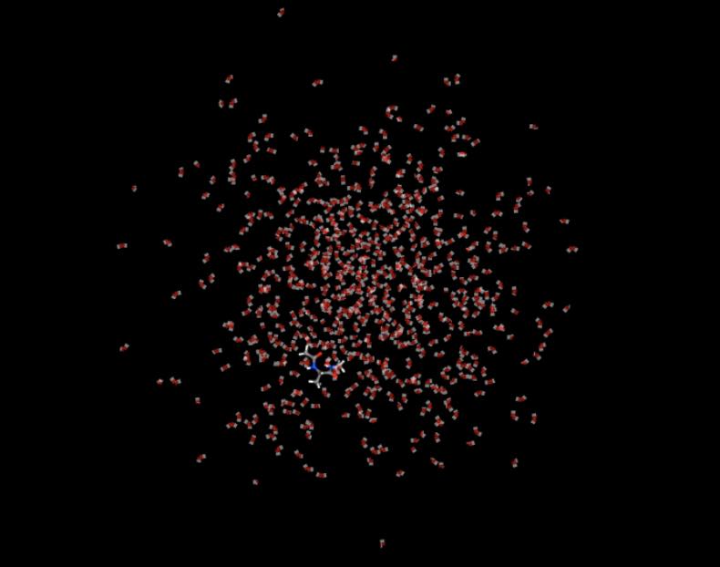
You can use any search term against any of the representations. For example, here we will do a more complex view of the aladip system where we render water molecules that are close to aladip differently to the rest of the water molecules in the box.

>>> mols = sr.load(sr.expand(sr.tutorial_url, "ala.top", "ala.crd"))
>>> mols.view(no_default=True,
...           surface="molidx 0",
...           spacefill="water within 5 of molidx 0",
...           ball_and_stick="water within 10 of molidx 0",
...           rest="line")

Note

Note how the distance calculation takes into account the periodic boundaries of the system. Note also that you can mix representation based views (e.g. surface="molidx 0") with search based views (e.g. rest="line").

Choosing colors and opacities

You can set the color and opacity used for a particular representation by passing these as additional terms to the representation or search term, separated by colons. For example, to set the color of a representation to blue we could pass this as an addition :blue to the representation or search term argument.

>>> mol = mols[0]
>>> mol.view(all="licorice:blue")

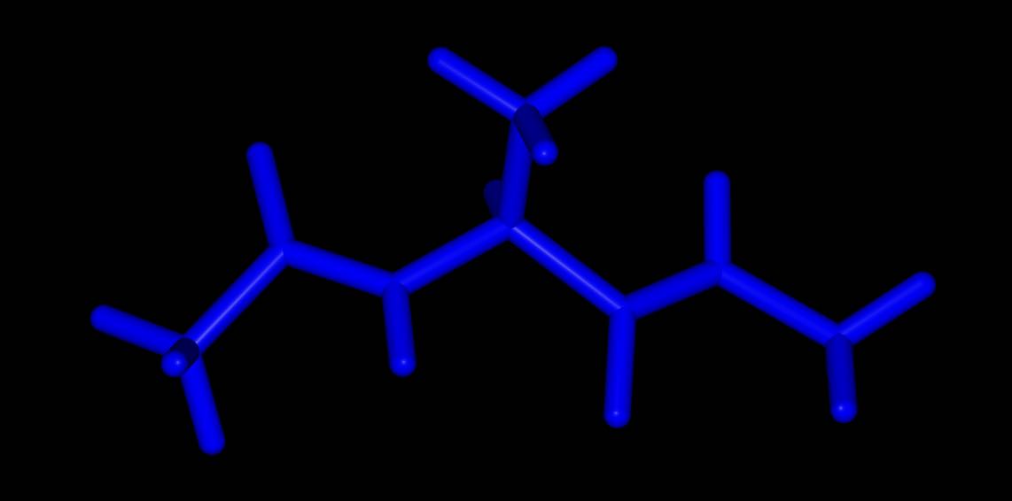
Here all of the atoms are rendered in blue licorice. Or…

>>> mol.view(all="licorice:blue", ball_and_stick="element C:red")

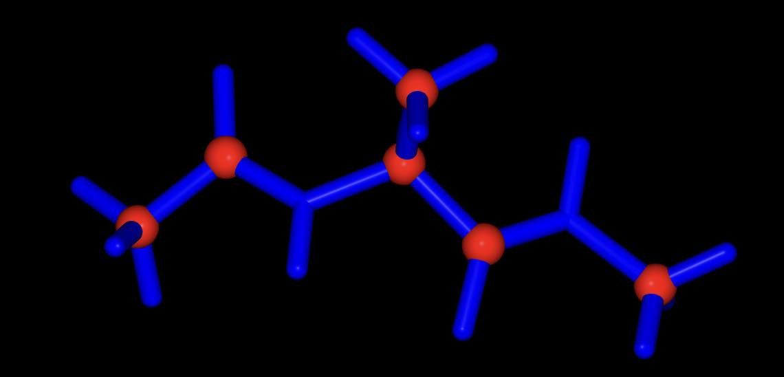
all of the atoms are rendered in blue licorice, but the carbon atoms are represented as red balls and sticks.

You can use any color name supported by NGLView. These include named colors (e.g. red, green, blue, yellow, including any CSS named color supported by your browser, e.g. orchid, sienna, wheat etc.), colors specified as a red-green-blue hex values (e.g. #FF0000, #00FF00, #0000FF etc.), colors specified as red-green-blue triples (e.g. rgb(255,0,0), rgb(0,255,0), rgb(0,0,255) etc.) or any of the coloring schemes supported by NGLView (e.g. atomindex, bfactor, electrostatic, element, hydrophobicity, random or sstruc).

You also specify the opacity (transparency) of the representation by adding a number between 0 (fully transparent) and 1 (fully opaque). You can use any order of color and opacity, e.g.

>>> mol.view(all=["licorice", "spacefill:0.8", "surface:red:0.2"])

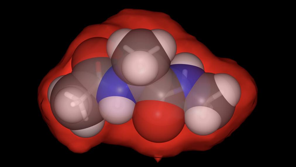
has rendered the molecule using three representations; a licorice in default colors (colored by element), spacefill in default colors, but with opacity 0.8, and a red-colored surface with opacity 0.2.

Or…

>>> mol.view(all=["ball_and_stick", "surface:0.9:electrostatic"])

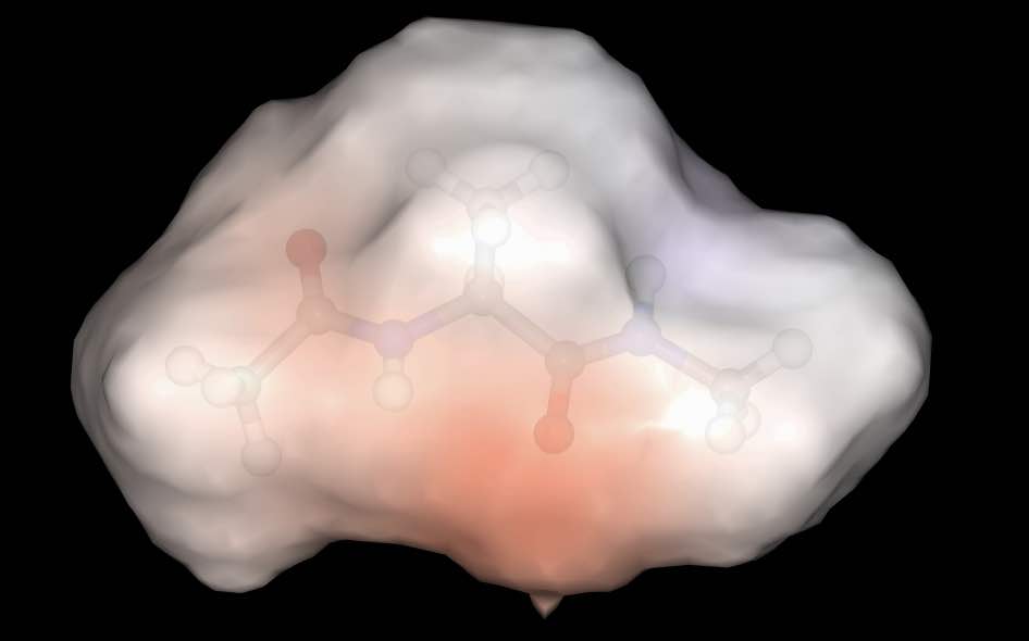
has rendered the molecule with two representations; a ball and stick with default colors and a surface colored using electrostatic potential, with opacity 0.9.

Centering the view

You can center the view on any selection using the center option, e.g.

>>> mols.view(center="molidx 0")

would center the view on the first molecule, or,

>>> mols.view(center="not (water or protein")

would center the view on all none (water, protein) molecules, i.e. likely any ligands or ions. Remember that you can create your own custom selections to set search terms that refer to ligands or ions more specifically.

Viewing trajectories

If the molecules being viewed have a trajectory, then you will also see play controls in the bottom left. These will let you play, pause and scroll through the trajectory. Click the play button multiple times to speed up playback.

You can choose a subset of frames to play, e.g. here we will play a movie of the first 10 frames of the trajectory.

>>> mols = sr.load(sr.expand(sr.tutorial_url, "ala.top", "ala.traj"))
>>> mols.trajectory()[0:10].view()

Or here we can view every 25 frames of the trajectory.

>>> mols.trajectory()[0::25].view()

Or here we can view all of the frames in reverse order

>>> mols.trajectory()[::-1].view()

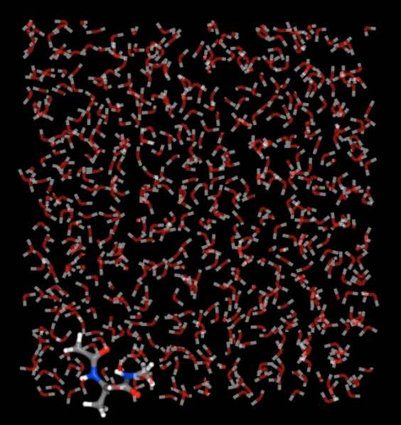
Wrapping molecules into the current box

You can control whether or not molecules are wrapped into the same periodic box using the wrap option. If this is True (the default), then the molecules are wrapped into the same box. If this is False then the wrapping will be whatever was loaded from the trajectory file (or generated via the simulation). For example, the trajectory is not wrapped, and so the water molecules will gradually drift out into neighboring boxes. You can see this by passing in wrap=False, e.g.

>>> mols.trajectory()[-1].view(wrap=False)

This compares to

>>> mols.trajectory()[-1].view(wrap=True)

Note

We are viewing the last frame here, as this is the one that shows the maximum amount of drift from the central box.

Trajectory Alignment

You can align the frames in a trajectory by passing in a search string via the align keyword. For example, here we could align every frame against all of the carbon atoms.

>>> mols.view(align="element C")

Note

You can also pass in a sub-view directly, e.g. mols.view(align=mols["element C"]).

If wrap is True (as is the default) then all molecules will be wrapped such that the aligned atoms are at the center of the box.

You can use any search string or view to find the atoms to align. If you pass align=True then this will align against all atoms. This can be useful when you are viewing individual molecules, e.g.

>>> mols[0].view(align=True)

Trajectory Smoothing

Molecular dynamics trajectories can be difficult to view because there is a lot of high frequency random motion that can obscure the low frequency conformational changes that are often of more interest. One way to view these events is to average the coordinates of atoms over several frames. You can do this using the smooth option, e.g.

>>> mols.view(align="element C", smooth=50)

Would align the trajectory using all carbon atoms, and would average the coordinates of each atom over 50 neighboring frames.

Note

The smoothing number, s is divided by two, with each frame being averaged over the previous (s/2)-1 preceeding frames and (s/2)+x following frames (where x is zero if s is even, and one otherwise).

Integration with trajectories

Note that all of the above options can be passed to the trajectory() function, e.g.

>>> mols.trajectory(align="element C", smooth=50).view()

would give the same view as

>>> mols.view(align="element C", smooth=50)

as would

>>> mols.trajectory(align=mols["element C"], smooth=50).view()

and

>>> mols.view(align=mols["element C"], smooth=50)

This is because mols.view(...) is creating its own mols.trajectory(...) with those options, and is viewing those.

While you can do this, and it is useful for, e.g. saving trajectories, there are lots of edge cases that could trip you up. We recommend that you pass the options to the view function and don’t pass them to the trajectory function when you want to view.

Note

The options passed to view will override those passed to trajectory, e.g. mols.trajectory(smooth=10).view(smooth=50) will use a smooth value of 50.

Note

The value of wrap in the view function defaults to True. This means that mols.trajectory(wrap=False).view() will wrap the coordinates, as the value of wrap in the view function defaults to True and overrides the value in trajectory. To show unwrapped, you would need to use mols.trajectory(wrap=False).view(wrap=False), or the much easier mols.trajectory().view(wrap=False), or the easiest mols.view(wrap=False).

Setting the background color

You can set the background color of the view using the bgcolor argument. This should be a string, using any color that is recognised by NGLView via the backgroundColor stage parameter.

>>> mols[0].view(bgcolor="black")

Note

The default background color is black.

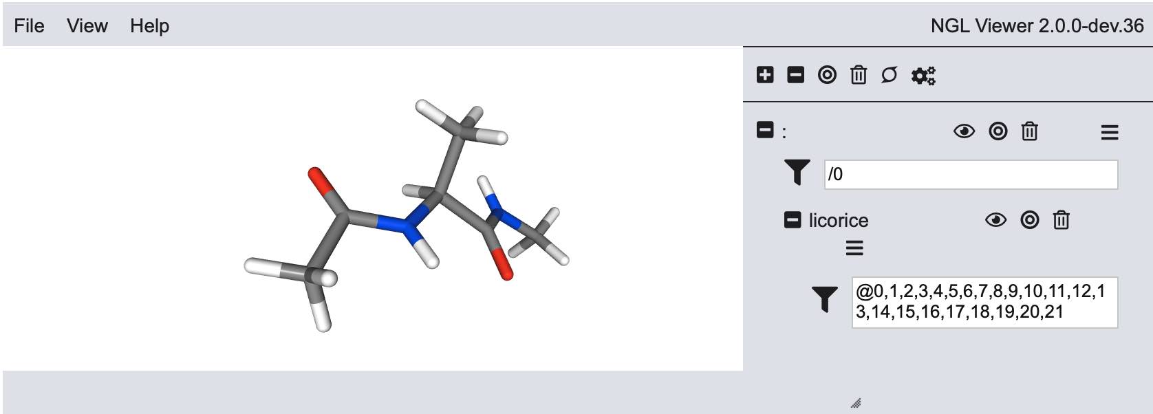
Closer integration with NGLView

We don’t yet properly expose the NGLView stage parameters. Currently you can pass in a dictionary of parameters via the stage_parameters argument, which are straight passed to the NGLView.NGLWidget.stage.

If you want more control over the view, you can assign the result of mols.view(...) to a variable. This variable is the actual NGLView.NGLWidget, which you can manipulate as if you had created it yourself, e.g.

>>> v = mols[0].view()
>>> v.stage.set_parameters(backgroundColor="white")
>>> v.display(gui=True)
>>> v.camera = "perspective"
>>> v

Saving 3D views to files

NGLView is not really designed to render frames via a script. Instead, it needs to be run within a Jupyter notebook so that it has access to the WebGL view in the web browser to perform the rendering. This FAQ answer shows how you could automate rendering images to files. Note that you need to get the handle to the NGLView.NGLWidget, as above, and then call render_image to get the image. You will need to actually view the object in a code cell, and will need to wait for the image to render, e.g. in one code cell

>>> v = mols.view()
>>> v

Then in the next

>>> def render(view, filename):
...    import time
...    image = view.render_image()
...
...    while not image.value:
...        time.sleep(0.1)
...
...    with open(filename, "wb") as f:
...        f.write(image.value)

and then finally, to call this function in a background thread…

>>> import threading
... thread = threading.Thread(
...     target=render,
...     args=(v, "image.png")
... )
>>> thread.daemon = True
>>> thread.start()