Trajectories
sire supports loading, editing and saving of trajectories via multiple
file formats. Trajectories are represented as a series of frames, with
each frame containing (optionally) coordinate, velocity, force, space,
time and generic property data.
Supported file formats
sire natively supports the following trajectory formats:
Format |
Parser |
Description |
|---|---|---|
DCD |
DCD coordinate/velocity binary trajectory files based on charmm / namd / x-plor format. |
|
RST |
Amber coordinate/velocity binary (netcdf) restart/trajectory files supported since Amber 9, now default since Amber 16. |
|
TRAJ |
Amber trajectory (ascii) coordinate or velocity files supported from Amber 7 upwards. |
|
TRR |
Gromacs TRR (XDR file) coordinate / velocity / force trajectory file |
|
XTC |
Gromacs XTC (XDR file) compressed coordinate trajectory file |
The DCD, RST and
TRR formats are binary, and so hold the trajectory
data at the highest precision and in the most compact format. They are
easily seekable, so give the best balance between speed and trajectory size.
The TRAJ format is text-based, and so takes up a
lot of space and stores data at a fixed (lower) precision. It is included
for completeness, but is not recommended as a format for saving new
trajectories.
The XTC is a compressed binary format that stores
trajectory data in binary in lower precision. This is very space efficient,
but at the cost of losing quite a bit of precision in the exact coordinate
data. It is only recommended if you want to save storage space and don’t
need to recover, e.g. energies or other properties that depend
on exact coordinates.
Loading trajectories
You load trajectories in the same way as loading any other file, e.g.
using sire.load().
>>> import sire as sr
>>> mols = sr.load(sr.expand(sr.tutorial_url, "ala.top", "ala.traj"))
>>> print(mols.num_frames())
500
sire will automatically determine the format of the trajectory.
For example, here we have loaded the 500 frames from the file
ala.traj. This file is in RST format, not
TRAJ format, despite the file extension.
An exception will be raised if any errors are detected in the trajectory files. These errors can sometimes be difficult to debug. To help, you can try to directly load the trajectory file using the appropriate parser, e.g.
>>> t = sr.io.parser.TRAJ("ala.traj")
UserWarning: SireIO::parse_error: Disagreement over the number of read bytes... 128 vs -13.
This indicates a program bug or IO error. (call sire.error.get_last_error_details()
for more info)
Trying using the correct parser gives us
>>> t = sr.io.parser.RST("ala.traj")
>>> t
AmberRst( nAtoms() = 1912, nFrames() = 500 )
You can use the parsers to read frames individually into
sire.mol.Frame objects, e.g.
>>> f = t.get_frame(0)
>>> print(f)
The Frame object has functions like .coordinates(),
.velocities() and .forces(), which can be used to get the
raw coordinates, velocities and forces data from the frame.
Loading and joining multiple trajectories
It is easy to load and join multiple trajectories together into a single
trajectory. You just load multiple files, in the order in which you
want the trajectory frames to be placed. Assuming you have trajectory
files block1.rst, block2.rst, block3.rst, with the topology
in file topology.prm, then you could load
them as a single trajectory via
>>> import sire as sr
>>> mols = sr.load("topology.prm", "block1.rst", "block2.rst", "block3.rst")
or, you could use file globbing, e.g.
>>> mols = sr.load("topology.prm", "block*.rst")
Note that you can load a combination of trajectories with different formats, e.g.
>>> mols = sr.load("topology.prm", "block1.rst", "block2.dcd", "block3.trr")
Saving trajectories
You can save trajectories using the sire.save() function. For example
>>> import sire as sr
>>> mols = sr.load(sr.expand(sr.tutorial_url, "ala.top", "ala.traj"))
>>> f = sr.save(mols, "output", format=["RST"])
>>> print(f)
["output.rst"]
>>> print(sr.io.parser.RST(f[0]))
AmberRst( nAtoms() = 1912, nFrames() = 1 )
would save the first frame of the trajectory loaded from ala.traj to
a RST format file called output.rst.
To save all the frames, you need to pass in a TrajectoryIterator
that specifies which frames to save. You can get the
TrajectoryIterator that specifies all frames just be
calling .trajectory() on the molecule(s) you want to save.
>>> f = sr.save(mols.trajectory(), "output", format=["RST"])
>>> print(sr.io.parser.RST(f[0]))
AmberRst( nAtoms() = 1912, nFrames() = 500 )
You can choose subsets of frames to save via the functions of the
TrajectoryIterator (typically using the indexing functions).
For example, here we can save frames 10-100 to TRR format.
>>> f = sr.save(mols.trajectory()[10:101], "output", format=["TRR"])
>>> print(sr.io.parser.TRR(f[0]))
TRR( nAtoms() = 1912, nFrames() = 91 )
or here we can save every 10th frame to DCD format.
>>> f = sr.save(mols.trajectory()[::10], "output", format=["DCD"])
>>> print(sr.io.parser.DCD(f[0]))
DCD( nAtoms() = 1912, nFrames() = 50 )
or here we will write all frames out in reverse order to
XTC format.
>>> f = sr.save(mols.trajectory()[::-1], "output", format=["XTC"])
>>> print(sr.io.parser.XTC(f[0]))
XTC( nAtoms() = 1912, nFrames() = 500 )
Saving trajectory for subsets of molecules
You can save trajectories for subsets of molecules, just be passing in
the TrajectoryIterator for that subset to
sire.save(). For example, here we will save every frame of the
first molecule in the system to TRAJ format.
>>> f = sr.save(mols[0].trajectory(), "output", format=["TRAJ"])
>>> print(sr.io.parser.TRAJ(f[0]))
AmberTraj( title() = TRAJ file create by sire, nAtoms() = 22, nFrames() = 500 )
Saving to multiple files in parallel
You can save a trajectory to as many files as you wish. For example, you
could simultaneously write the trajectory to
RST and DCD format by passing
in both RST and DCD to the format argument.
>>> f = sr.save(mols.trajectory(), "output", format=["RST", "DCD"])
>>> print(f)
["output.rst", "output.dcd"]
It is also common to save the topology for the trajectory at the same time,
particular as this makes loading it in the future easier. Here we will
save the trajectory as a Gromacs topology and DCD
file.
>>> f = sr.save(mols.trajectory(), "output", format=["GroTop", "DCD"])
>>> print(f)
["output.grotop", "output.dcd"]
>>> mols = sr.load(f, silent=True)
>>> print(mols, mols.num_frames())
System( name=ACE num_molecules=631 num_residues=633 num_atoms=1912 ) 500
Note
You can mix and match topology and trajectory formats, e.g. save Amber PRM topologies with Gromacs TRR trajectories. You don’t need to choose “compatible” formats.
Saving to file trajectories
In addition to the standard trajectory formats, sire also supports
reading and writing coordinates to single-frame formats, e.g.
PDB, SDF etc.
These “single-frame” formats are not really designed to hold multiple
frames of a trajectory. To support these formats, sire will write
trajectories for these formats as a collection of individual frame files
within a directory named according to the output file. For example,
here we will write every 10th frame as a PDB` file,
and will also write the topology to a PRM file.
>>> f = sr.save(mols.trajectory()[::10], "output", format=["PRM", "PDB"])
>>> print(f)
["output.prm", "output.pdb"]
This output.pdb is actually a directory that contains individual PDB
files for each frame, e.g.
>>> import os
>>> os.listdir("output.pdb")
['frame_049_98.pdb',
 'frame_040_80.pdb',
 'frame_002_4.pdb',
 'frame_042_84.pdb',
 'frame_024_48.pdb',
...
 'frame_045_90.pdb',
 'frame_004_8.pdb',
 'frame_034_68.pdb']
Each frame’s filename includes the frame number (e.g. 49 for the first
frame listed above) and the time in picoseconds (98 ps) of that frame.
You can load all of these frames by just passing in the name of the directory (together with a topology file), e.g.
>>> mols = sr.load("output.prm", "output.pdb")
>>> print(mols, mols.num_frames())
System( name=ACE num_molecules=631 num_residues=633 num_atoms=1912 ) 50
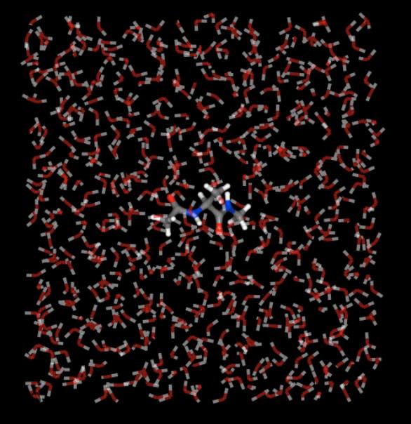
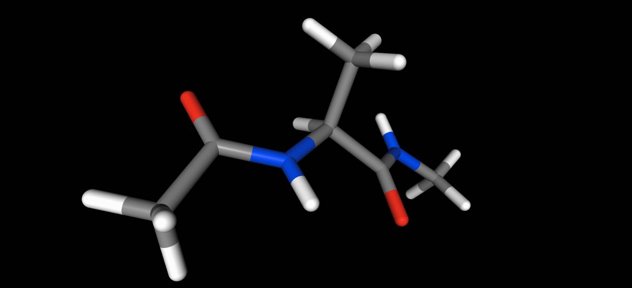
Visualising trajectories
Viewing trajectories is very simple - just call .view() on any
view of molecules that contains a trajectory.
>>> import sire as sr
>>> mols = sr.load(sr.expand(sr.tutorial_url, "ala.top", "ala.traj"))
>>> mols.view()
Use the “play” button or trajectory slider to move through the trajectory.
You can view sub-frames or sub-sets of the trajectory by calling
.view() on those sub-sets, or by passing in
a TrajectoryIterator that contains the frames you
want to view. For example, this would view the trajectory of just
the first molecule.
>>> mols[0].view()
While this would view every 10 frames of the trajectory.
>>> mols.trajectory()[::10].view()
See the view documentation for more information on how you can control the view.
Smoothing and aligning frames
sire has in-built support for processing trajectories. You can
re-wrap molecules into periodic boxes, align frames against a selection,
and also average (smooth) coordinates across multiple frames.
For example, here we will align all frames against the selection of carbon atoms.
>>> import sire as sr
>>> mols = sr.load(sr.expand(sr.tutorial_url, "ala.top", "ala.traj"))
>>> mols.view(align="element C")
or
>>> mols.view(align=mols["element C"])
And here we will smooth trajectories by averaging over 20 frames
>>> mols.view(smooth=20)
Here we center the view on the first molecule
>>> mols.view(center="molidx 0")
and here we turn off automatic wrapping of molecules into the periodic box
>>> mols.view(wrap=False)
You can use similar arguments to save the results of this processing to a trajectory file. So,
>>> f = sr.save(mols.trajectory(smooth=20), "smoothed", format=["RST"])
saves the results of smoothing the trajectory over 20 frames to the
file smoothed.rst.
Similarly
>>> f = sr.save(mols.trajectory(align="element C"), "aligned", format=["DCD"])
or
>>> f = sr.save(mols.trajectory(align=mols["element C"], "aligned", format=["DCD"]))
saves the result of aligning every frame against carbon atoms to a
file aligned.dcd,
while
>>> f = sr.save(mols.trajectory(wrap=False), "not_wrapped", format=["TRR"])
saves the trajectory without wrapping into the periodic space to the
file not_wrapped.trr.
To automatically wrap the frames use
>>> f = sr.save(mols.trajectory(wrap=True), "wrapped", format=["TRR"])
Note
Viewing molecules will automatically wrap into the periodic box
(so for .view(), the value of wrap defaults to True).
In contrast, saving molecules will not automatically wrap into the
periodic box (so for sire.save, the value of wrap defaults
to False). This is because you typically want to wrap
coordinates when viewing trajectories, while you typically don’t
want the code to change the wrapping state of a trajectory when you
save it (i.e. you don’t want an unwrapped trajectory that was loaded
to be automatically wrapped on save). Make sure that you set the
value of wrap if you want to ensure a particular behaviour.
Aligning to molecules outside the trajectory
You can also align to molecules that are not part of a trajectory. You
do this by giving a view of the reference molecules againt
which to align the trajectory, and also supplying
an sire.mol.AtomMapping object that describes how atoms in
the reference map to atoms in the trajectory.
For example, imagine you have loaded the same molecule in two files.
>>> import sire as sr
>>> mols = sr.load(sr.expand(sr.tutorial_url, "ala.top", "ala.traj"))
>>> ref_mols = sr.load(sr.expand(sr.tutorial_url, "ala.top", "ala.crd"))
You could align the trajectory in mols against the molecules in
ref_mols by building a mapping. For example, the mapping could be
between the alanine dipeptide molecule in both trajectories. You can
build the mapping using the sire.match_atoms() function.
>>> mapping = sr.match_atoms(ref_mols[0], mols[0], match_light_atoms=True)
Now you can align mols against ref_mols by passing in this mapping,
e.g.
>>> f = sr.save(mols.trajectory(align=ref_mols[0], mapping=mapping), "aligned", format=["DCD"])
You could also use mappings to calculate RMSDs against this molecule, e.g.
>>> mols.trajectory().rmsd(ref_mols[0], mapping=mapping)
or when viewing the trajectory
>>> mols.view(align=ref_mols[0], mapping=mapping)
Calculating energies across frames
You can perform lots of different types of analysis across trajectory frames.
A useful type of analysis is calculating the interaction energy between
molecules. For example, you could use the .energy() function to calculate
total energies of each frame,
>>> import sire as sr
>>> mols = sr.load(sr.expand(sr.tutorial_url, "ala.top", "ala.traj"))
>>> print(mols.trajectory().energy())
     frame        time    1-4_LJ  1-4_coulomb          LJ      angle      bond      coulomb   dihedral  improper  intra_LJ  intra_coulomb        total
0        0    0.200000  3.509838    44.810452  922.010757   7.570059  4.224970 -6794.775454   9.800343  0.485545 -1.311255     -37.520806 -5841.195551
1        1    0.400000  2.700506    47.698455  928.715959  12.470519  2.785875 -6861.966370  11.776295  1.131481 -1.617496     -40.126219 -5896.430994
2        2    0.600000  2.801076    43.486411  838.387490  11.607753  2.023439 -6724.278286  11.614774  0.124729 -1.103966     -36.633297 -5851.969876
3        3    0.800000  3.365638    47.483966  958.913012   6.524609  0.663455 -6828.029775  11.383852  0.339333 -0.983872     -40.197920 -5840.537702
4        4    1.000000  3.534830    48.596027  915.994574   6.517530  2.190370 -6838.160251  10.214994  0.255331 -1.699613     -40.355054 -5892.911262
..     ...         ...       ...          ...         ...        ...       ...          ...        ...       ...       ...            ...          ...
495    495   99.199997  2.665994    42.866319  899.586671  11.339087  4.172684 -6636.461269   9.875872  0.356887 -1.584092     -36.499764 -5703.681610
496    496   99.400002  3.062467    44.852774  916.416899   9.268408  1.878366 -6582.928689  10.548897  0.327064 -1.814718     -36.671683 -5635.060214
497    497   99.599998  3.530233    44.908117  895.229707  10.487378  4.454670 -6600.333270  10.223964  1.006034 -0.692972     -37.118048 -5668.304187
498    498   99.800003  3.511116    42.976288  851.153213   9.017446  0.809064 -6557.430299  10.841436  0.518190 -1.862433     -35.481467 -5675.947445
499    499  100.000000  3.768998    41.625135  825.743725  13.629923  1.089917 -6504.532783  11.889372  0.846805 -1.897328     -36.547672 -5644.383908
[500 rows x 13 columns]
Or you could calculate the interaction energy between the first molecule and all of the water molecules.
>>> print(mols[0].trajectory().energy(mols["water"]))
     frame        time         LJ    coulomb      total
0        0    0.200000 -16.380889 -35.380162 -51.761051
1        1    0.400000  -8.945872 -36.624766 -45.570638
2        2    0.600000 -17.827446 -27.348159 -45.175605
3        3    0.800000 -17.448833 -34.799090 -52.247922
4        4    1.000000 -12.476675 -43.806890 -56.283565
..     ...         ...        ...        ...        ...
495    495   99.199997 -10.742225 -36.700127 -47.442352
496    496   99.400002 -14.539061 -29.326716 -43.865778
497    497   99.599998 -10.165851 -35.616962 -45.782813
498    498   99.800003 -12.226096 -35.170080 -47.396176
499    499  100.000000  -7.356142 -41.265345 -48.621487
[500 rows x 5 columns]
Trajectories and PageCache
When you run a molecular dynamics simulation, you will typically generate
a lot of frames, which will become too large to fit in memory. To handle
this, a sire.base.PageCache is used. This class provides a
PageCache to which objects can be stored and fetched.
The memory for those objects is automatically paged back to disk, meaning
that it doesn’t need to stay resident in memory.
The System class automatically uses a
PageCache to manage the frames involved in its
save_frame() and
load_frame() function calls. This page cache
will page data larger than ~256MB to disk, into a directory called
temp_trajectory_XXXXXX in the current working directory
(where XXXXXX is replaced with a random string). This directory
will be automatically cleaned up when the program exits, and potentially
earlier when the system is deleted and then garbage collected by python.
You can change the location of the page cache in two ways. Either,
you can set the environment variable SIRE_PAGECACHE_ROOT to the directory
where you want the page cache to be stored, or you can call the
set_root_directory() function to set the
root directory in your script.
You can also use the PageCache class directly to
create caches for your own objects. For example, here we will create a
cache into which we will place some data.
>>> import sire as sr
>>> cache = sr.base.PageCache()
>>> handle1 = cache.store("Hello World")
>>> mols = sr.load_test_files("ala.top", "ala.crd")
>>> handle2 = cache.store(mols)
>>> print(handle1.fetch())
Hello World
>>> print(handle2.fetch())
System( name=ACE num_molecules=631 num_residues=633 num_atoms=1912 )
>>> print(sr.base.PageCache.get_statistics())
Cache: /path/to/cache_root/temp_XXXXXX
  Current Page: 977.279 KB : is_resident 1
  Total size: 977.279 KB
Note
The PageCache class can hold any object that is
picklable.