Alanine-dipeptide conformational landscape

Note

The code in this tutorial was adapted from FastMBAR.

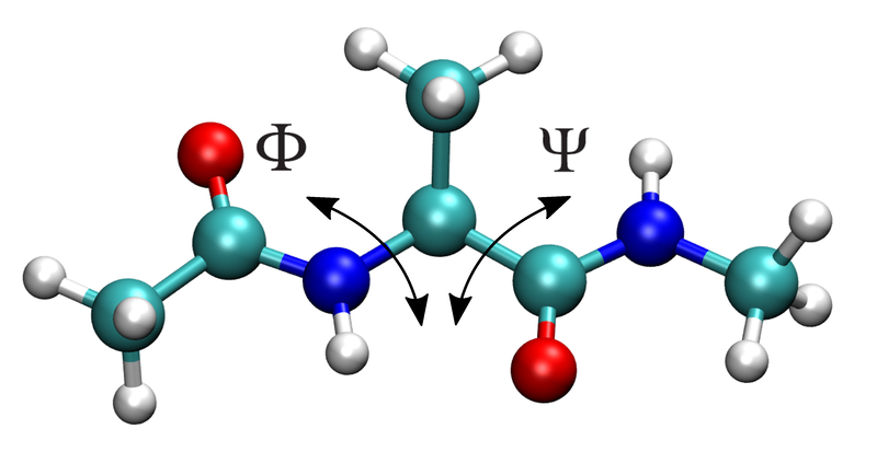
In a recent preprint we used the emle-engine interface to sander to compute free-energy surfaces for alanine-dipeptide as a function of the Φ and Ψ dihedral angles shown below. Compared to regular mechanical embedding, EMLE was found to be closer to the reference density-functional theory (DFT) surface. In this tutorial we will show how to use the sire-emle interface to set up and run the same calculations using OpenMM.

Creating a context with sire-emle

As in the previous section, we can first use sire-emle to create a QM/MM capable dynamics object for the alanine-dipeptide example system. We can then extract the underlying OpenMM context from this.

First we will create an EMLECalculator to compute the QM intramolecular interaction using ANI-2x along with the electrostatic embedding interaction.

>>> from emle import EMLECalculator
>>> calculator = EMLECalculator(device="cpu")

Next we will load the alanine-dipeptide system using sire:

>>> import sire as sr
>>> mols = sr.load_test_files("ala.crd", "ala.top")

We can then create an EMLEEngine that can be be used to perform QM/MM:

>>> qm_mols, engine = sr.qm.emle(mols, mols[0], calculator)

Here the first argument is the molecules that we are simulating, the second selection coresponding to the QM region (here this is the first molecule), and the third is calculator that was created above. The fourth and fifth arguments are optional, and specify the QM cutoff distance and the neigbour list update frequency respectively. (Shown are the default values.) The function returns a modified version of the molecules containing a “merged” dipeptide that can be interpolated between MM and QM levels of theory, along with an engine. The engine registers a Python callback that uses emle-engine to perform the QM calculation.

We can now create a dynamics that will create an OpenMM context for us and can be used to run a simulation:

>>> d = mols.dynamics(
...     timestep="1fs",
...     constraint="none",
...     engine=engine,
...     platform="cpu",
... )

Before extracting the context we will use the dynamics object to minimise the alanine-dipeptide system:

>>> d.minimise()

Setting up umbrella sampling with OpenMM

We can now extract the underlying OpenMM context from the dynamics object, then create a copy of the integrator and system.

>>> from copy import deepcopy
>>> context = d.context()
>>> omm_system = context.getSystem()
>>> integrator = deepcopy(context.getIntegrator())

In order to perform umbrella sampling we will need to add a biasing potentials for the two dihedral angles. Here we will use simple harmonic biasing potentials:

First the Φ dihedral, which is formed by atom indices 4, 6, 8, and 14:

>>> import openmm
>>> import openmm.app
>>> bias_torsion_phi = openmm.CustomTorsionForce(
...     "0.5*k_phi*dtheta^2; dtheta = min(tmp, 2*pi-tmp); tmp = abs(theta - phi)"
... )
>>> bias_torsion_phi.addGlobalParameter("pi", math.pi)
>>> bias_torsion_phi.addGlobalParameter("k_phi", 100.0)
>>> bias_torsion_phi.addGlobalParameter("phi", 0.0)
>>> bias_torsion_phi.addTorsion(4, 6, 8, 14)

Next the Ψ dihedral, which is formed by atom indices 6, 8, 14, and 16:

>>> bias_torsion_psi = openmm.CustomTorsionForce(
...     "0.5*k_psi*dtheta^2; dtheta = min(tmp, 2*pi-tmp); tmp = abs(theta - psi)"
... )
>>> bias_torsion_psi.addGlobalParameter("pi", math.pi)
>>> bias_torsion_psi.addGlobalParameter("k_psi", 100.0)
>>> bias_torsion_psi.addGlobalParameter("psi", 0.0)
>>> bias_torsion_psi.addTorsion(6, 8, 14, 16)

We can now add these forces to the system:

>>> omm_system.addForce(bias_torsion_phi)
>>> omm_system.addForce(bias_torsion_psi)

In order to run the simulation we will create a new context using the system and integrator and set the initial positions.

>>> new_context = openmm.Context(omm_system, integrator, context.getPlatform())
>>> new_context.setPositions(context.getState(getPositions=True).getPositions())

Running the simulation

We are almost ready to run an umbrella sampling simulation. In this example we will sample the Φ and Ψ dihedral angles on a 36x36 grid. We will first set the biasing potential centers:

>>> m = 36
>>> M = m * m
>>> phi = np.linspace(-math.pi, math.pi, m, endpoint=False)
>>> psi = np.linspace(-math.pi, math.pi, m, endpoint=False)

During the simulation we will save trajectories to disk which can later be post-processed to compute the dihedral angles. We will create a directory in which to store the files:

>>> os.makedirs("./output/traj", exist_ok=True)

The sampling is performed by looping over each of the umbrella windows sequentially. For each window we set the biasing potential center and run an initial equilibration of 5000 steps. We then run a production simulation of 100 cycles of 100 steps each, saving trajectory after each cycle:

>>> for idx in range(M):
... phi_index = idx // m
... psi_index = idx % m
...
... # Set the center of the biasing potentials.
... new_context.setParameter("phi", phi[phi_index])
... new_context.setParameter("psi", psi[psi_index])
...
... # Initial equilibrium.
... integrator.step(5000)
...
... # Production sampling.
... file_handle = open(f"./output/traj/phi_{phi_index}_phi_{psi_index}.dcd", "bw")
... dcd_file = DCDFile(file_handle, prm.topology, dt=integrator.getStepSize())
... for x in range(100):
...     integrator.step(100)
...     state = new_context.getState(getPositions=True)
...     positions = state.getPositions()
...     dcd_file.writeModel(positions)
... file_handle.close()

Note

This is not a particulary efficient way to perform the sampling. In practice, since it’s possible to get good single core performance it is better to run the windows in parallel, either individually, or in blocks.

Analysing the results

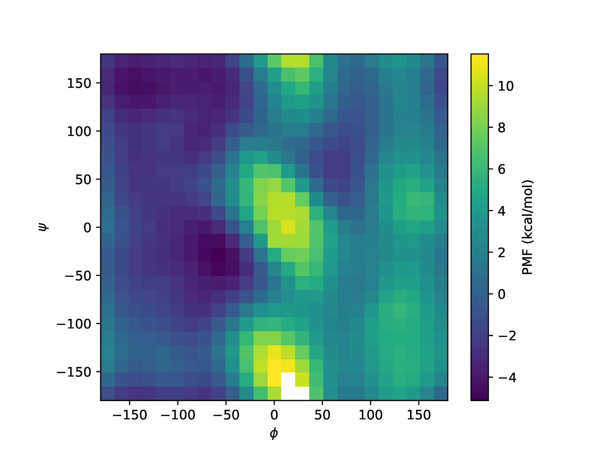
The trajectories saved to disk can be post-processed to compute the dihedral angles, for example using the approach here. The free-energy surface can then be compute using MBAR, or UWHAM. Example code is provided in the FastMBAR tutorial.

The resulting free-energy surface should look similar to the one shown below: