Running a Free Energy Perturbation Simulation
Now that you have your (possibly restrained) alchemical system, you can
run a free energy perturbation simulation. There are many ways to do this,
and the exact protocol will depend on what type of free energy you are
calculating, what level of accuracy you require and what compute resource
you have available. sire provides the building blocks to run a
simulation in any way you like, but in this tutorial we will use the
a very simple protocol. Take a look at
BioSimSpace or the upcoming
somd2 software if you are
interested in higher-level interfaces to this functionality that
automatically run more complex protocols.
At its simplest, a free energy perturbation simulation consists of a series of alchemical molecular dynamics simulations run at different values of the alchemical parameter, λ. Let’s start with the ethane to methanol merged molecule from the previous section.
>>> import sire as sr
>>> mols = sr.load(sr.expand(sr.tutorial_url, "merged_molecule.s3"))
>>> print(mols)
System( name=BioSimSpace_System num_molecules=4054 num_residues=4054 num_atoms=12167 )
And lets link the properties to the reference state, so that we start the simulation using the reference state coordinates.
>>> mols = sr.morph.link_to_reference(mols)
Next we will run through 21 evenly-space λ values from 0 to 1. We’ve picked 21 because it is a reasonable number that should over-sample the λ-coordinate.
For each λ-value, we will minimise the system, generate random velocities from a Boltzmann distribution for the simulation temperature, equilibrate the molecules for 2 ps, then run dynamics for 25 ps. We will calculate the energy of each simulation at each λ-value, plus at the neighbouring λ-values. This will allow us to calculate energy differences which we will later use to calculate the free energy difference.
We will calculate these energies every 0.1 ps, and will write them at the
end of each block of dynamics via the EnergyTrajectory
output which we will stream as a sire object.
This will let us subsequently calculate the free energy across λ using alchemlyb.
>>> for l in range(0, 105, 5):
...     # turn l into the lambda value by dividing by 100
...     lambda_value = l / 100.0
...     print(f"Simulating lambda={lambda_value:.2f}")
...     # minimise the system at this lambda value
...     min_mols = mols.minimisation(lambda_value=lambda_value).run().commit()
...     # create a dynamics object for the system
...     d = min_mols.dynamics(timestep="1fs", temperature="25oC",
...                           lambda_value=lambda_value)
...     # generate random velocities
...     d.randomise_velocities()
...     # equilibrate, not saving anything
...     d.run("2ps", save_frequency=0)
...     print("Equilibration complete")
...     print(d)
...     # get the values of lambda for neighbouring windows
...     lambda_windows = [lambda_value]
...     if lambda_value > 0:
...         lambda_windows.insert(0, (l-5)/100.0)
...     if lambda_value < 1:
...         lambda_windows.append((l+5)/100.0)
...     # run the dynamics, saving the energy every 0.1 ps
...     d.run("25ps", energy_frequency="0.1ps", frame_frequency=0,
...           lambda_windows=lambda_windows)
...     print("Dynamics complete")
...     print(d)
...     # stream the EnergyTrajectory to a sire save stream object
...     sr.stream.save(d.commit().energy_trajectory(),
...                    f"energy_{lambda_value:.2f}.s3")
This is a very simple protocol for a free energy simulation, with simulation times chosen so that it will run relatively quickly. For example, with a modern GPU this should run at about 60 nanoseconds of sampling per day, so take only 45 seconds or so for each of the 21 λ-windows.
Note
This is not enough sampling to calculate a properly converged free energy for most molecular systems. You would need to experiment with different equilibration and simulation times, or use a more sophisticated algorithm implemented via BioSimSpace or somd2.
Note
We set the forwards and backwards λ-values to (l-5)/100.0 and
(l+5)/100.0 so that they exactly match the way we set the reference
λ-value. This is because alchemlyb matches energies using a
floating point representation of λ, so small numerical differences
between, e.g. (l+5)/100.0 and lambda_value + 0.05 will lead
to errors (as in this case, (l+5)/100.0 is exactly every 0.05, while
lambda_value + 0.05 has numerical error, meaning some values are
at, e.g. 0.15000000000000002).
At the end of the simulation, you should have 21 energy files, one for each
λ-window. These are called energy_0.00.s3, energy_0.05.s3, …,
energy_1.00.s3.
Processing Free Energy Data using alchemlyb
alchemlyb is a simple alchemistry python package for easily analysing the results of free energy simulations. They have excellent documentation on their website that you can use if you want to go into the details of how to calculate free energies.
Here, we will show a simple BAR analysis of the data that we have just generated. We can do this because we have calculated data which alchemlyb can convert into reduced potentials for each λ-window.
First, we need to import alchemlyb
>>> import alchemlyb
Note
If you see an error then you may need to install (or reinstall)
alchemlyb. You can do this using conda e.g.
conda install -c conda-forge alchemlyb.
Next, we will load all of the EnergyTrajectory objects
for each λ-window, and will convert them into pandas DataFrames arranged
into an alchemlyb-compatible format. We could do this manually by first
loading all of the s3 files containing the EnergyTrajectory
objects…
>>> import sire as sr
>>> from glob import glob
>>> dfs = []
>>> energy_files = glob("energy*.s3")
>>> energy_files.sort()
>>> for energy_file in energy_files:
...     dfs.append(sr.stream.load(energy_file).to_alchemlyb())
Note
If you wanted, you could have put the dataframes generated above
directly into the dfs list here, and not saved them to disk
via the .s3 files. However, this would risk you having to re-run
all of the simulation if you wanted to change the analysis below.
Note
Be careful to load the DataFrames in λ-order. The glob function
can return the files in a random order, hence why we need to sort
this list. This sort only works because we have used a naming convention
for the files that puts them in λ-order. They must be in the right
order or else alchemlyb will calculate the free energy incorrectly
(it uses the column-order rather than the λ-order when calculating
free energies).
…then joining them together all of these DataFrames into a single DataFrame…
>>> import pandas as pd
>>> df = pd.concat(dfs)
>>> print(df)
                         0.00          0.05  0.10  0.15  0.20  0.25  0.30  0.35  ...  0.65  0.70  0.75  0.80  0.85  0.90          0.95          1.00
time fep-lambda                                                                  ...
2.1  0.0        -39300.750665 -39301.636585   NaN   NaN   NaN   NaN   NaN   NaN  ...   NaN   NaN   NaN   NaN   NaN   NaN           NaN           NaN
2.2  0.0        -39231.737759 -39232.504175   NaN   NaN   NaN   NaN   NaN   NaN  ...   NaN   NaN   NaN   NaN   NaN   NaN           NaN           NaN
2.3  0.0        -38982.663906 -38982.683430   NaN   NaN   NaN   NaN   NaN   NaN  ...   NaN   NaN   NaN   NaN   NaN   NaN           NaN           NaN
2.4  0.0        -38950.308505 -38950.357904   NaN   NaN   NaN   NaN   NaN   NaN  ...   NaN   NaN   NaN   NaN   NaN   NaN           NaN           NaN
2.5  0.0        -38732.275522 -38733.221193   NaN   NaN   NaN   NaN   NaN   NaN  ...   NaN   NaN   NaN   NaN   NaN   NaN           NaN           NaN
...                       ...           ...   ...   ...   ...   ...   ...   ...  ...   ...   ...   ...   ...   ...   ...           ...           ...
26.6 1.0                  NaN           NaN   NaN   NaN   NaN   NaN   NaN   NaN  ...   NaN   NaN   NaN   NaN   NaN   NaN -37208.485229 -37208.880770
26.7 1.0                  NaN           NaN   NaN   NaN   NaN   NaN   NaN   NaN  ...   NaN   NaN   NaN   NaN   NaN   NaN -37332.051194 -37332.476611
26.8 1.0                  NaN           NaN   NaN   NaN   NaN   NaN   NaN   NaN  ...   NaN   NaN   NaN   NaN   NaN   NaN -37276.392733 -37276.609020
26.9 1.0                  NaN           NaN   NaN   NaN   NaN   NaN   NaN   NaN  ...   NaN   NaN   NaN   NaN   NaN   NaN -37234.238097 -37234.603762
27.0 1.0                  NaN           NaN   NaN   NaN   NaN   NaN   NaN   NaN  ...   NaN   NaN   NaN   NaN   NaN   NaN -37268.684798 -37269.319345
Note
Do not worry about the large number of NaN values. These just show that
we have only calculated free energy differences along the diagonal of this
DataFrame, i.e. only between the simulated and neighbouring λ-windows.
…or we can use the in-build sire.morph.to_alchemlyb() function to
do all of the above for us.
>>> df = sr.morph.to_alchemlyb("energy*.s3")
This function is not only quicker, but it will automatically sort the data by λ-value, meaning that you don’t need to worry about the naming convention of your files.
Now we can tell alchemlyb to calculate the free energy using the BAR method.
>>> from alchemlyb.estimators import BAR
>>> b = BAR()
>>> b.fit(df)
>>> print(b.delta_f_.loc[0.00, 1.00])
-3.009332126465953
You can get a convergence plot, showing how the free energy changes as
a function of the simulation length using the convergence_plot function.
>>> from alchemlyb.convergence import forward_backward_convergence
>>> from alchemlyb.visualisation import plot_convergence
>>> f = forward_backward_convergence(dfs, "bar")
>>> plot_convergence(f)
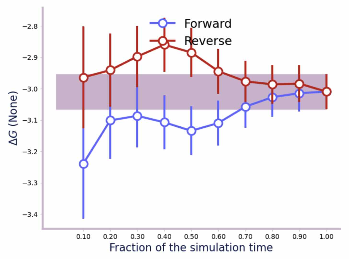
All of this shows that the relative free energy for the perturbation of ethane to methanol in water is about -3.0 kcal mol-1.
To get the relative hydration free energy, we would need to complete the
cycle by calculating the relative free energy for the perturbation in the
gas phase. We could do this using this code (which is almost identical to
above, except we only simulate the perturbable molecule, and save
the EnergyTrajectory objects to energy_gas_{lambda}.s3
instead of energy_{lambda}.s3).
>>> import sire as sr
>>> mols = sr.load(sr.expand(sr.tutorial_url, "merged_molecule.s3"))
>>> mol = mols.molecule("molecule property is_perturbable")
>>> mol = sr.morph.link_to_reference(mol)
>>> for l in range(0, 105, 5):
...     # turn l into the lambda value by dividing by 100
...     lambda_value = l / 100.0
...     print(f"Simulating lambda={lambda_value:.2f}")
...     # minimise the system at this lambda value
...     min_mol = mol.minimisation(lambda_value=lambda_value,
...                                vacuum=True).run().commit(return_as_system=True)
...     # create a dynamics object for the system
...     d = min_mol.dynamics(timestep="1fs", temperature="25oC",
...                          lambda_value=lambda_value,
...                          vacuum=True)
...     # generate random velocities
...     d.randomise_velocities()
...     # equilibrate, not saving anything
...     d.run("2ps", save_frequency=0)
...     print("Equilibration complete")
...     print(d)
...     # get the values of lambda for neighbouring windows
...     lambda_windows = [lambda_value]
...     if lambda_value > 0:
...         lambda_windows.insert(0, (l-5)/100.0)
...     if lambda_value < 1:
...         lambda_windows.append((l+5)/100.0)
...     # run the dynamics, saving the energy every 0.1 ps
...     d.run("25ps", energy_frequency="0.1ps", frame_frequency=0,
...           lambda_windows=lambda_windows)
...     print("Dynamics complete")
...     print(d)
...     # stream the EnergyTrajectory to a sire save stream object
...     sr.stream.save(d.commit().energy_trajectory(),
...                    f"energy_gas_{lambda_value:.2f}.s3")
Note
The option vacuum=True tells the minimisation and dynamics to
remove any simulation space that may be attached to the molecule(s),
and instead set the space to a Cartesian space.
This has the affect of simulating the molecules in vacuum.
Note
The option return_as_system tells the minimisation’s commit
function to return the result as a System object,
rather than a molecule. This way, min_mol is a System,
and so you can access the energy trajectory via the
energy_trajectory() function.
This should run more quickly than the simulation in water, e.g. about 15 seconds per window (at about 150 nanoseconds per day of sampling).
We can then analyse the results using the same analysis code, except we
switch to analysing the energy_gas_{lambda}.s3 files instead.
>>> df = sr.morph.to_alchemlyb("energy_gas*.s3")
>>> print(df)
                     0.00      0.05  0.10  0.15  0.20  0.25  0.30  0.35  0.40  ...  0.60  0.65  0.70  0.75  0.80  0.85  0.90      0.95      1.00
time fep-lambda                                                                ...
2.1  0.0         6.966376  7.115377   NaN   NaN   NaN   NaN   NaN   NaN   NaN  ...   NaN   NaN   NaN   NaN   NaN   NaN   NaN       NaN       NaN
2.2  0.0         6.614100  6.434525   NaN   NaN   NaN   NaN   NaN   NaN   NaN  ...   NaN   NaN   NaN   NaN   NaN   NaN   NaN       NaN       NaN
2.3  0.0         6.782235  6.831925   NaN   NaN   NaN   NaN   NaN   NaN   NaN  ...   NaN   NaN   NaN   NaN   NaN   NaN   NaN       NaN       NaN
2.4  0.0         4.196341  4.227257   NaN   NaN   NaN   NaN   NaN   NaN   NaN  ...   NaN   NaN   NaN   NaN   NaN   NaN   NaN       NaN       NaN
2.5  0.0         4.141862  4.205784   NaN   NaN   NaN   NaN   NaN   NaN   NaN  ...   NaN   NaN   NaN   NaN   NaN   NaN   NaN       NaN       NaN
...                   ...       ...   ...   ...   ...   ...   ...   ...   ...  ...   ...   ...   ...   ...   ...   ...   ...       ...       ...
26.6 1.0              NaN       NaN   NaN   NaN   NaN   NaN   NaN   NaN   NaN  ...   NaN   NaN   NaN   NaN   NaN   NaN   NaN  8.246601  8.707174
26.7 1.0              NaN       NaN   NaN   NaN   NaN   NaN   NaN   NaN   NaN  ...   NaN   NaN   NaN   NaN   NaN   NaN   NaN  7.169596  7.100342
26.8 1.0              NaN       NaN   NaN   NaN   NaN   NaN   NaN   NaN   NaN  ...   NaN   NaN   NaN   NaN   NaN   NaN   NaN  6.422485  6.466972
26.9 1.0              NaN       NaN   NaN   NaN   NaN   NaN   NaN   NaN   NaN  ...   NaN   NaN   NaN   NaN   NaN   NaN   NaN  5.892950  6.129184
27.0 1.0              NaN       NaN   NaN   NaN   NaN   NaN   NaN   NaN   NaN  ...   NaN   NaN   NaN   NaN   NaN   NaN   NaN  7.487893  7.618827
>>> from alchemlyb.estimators import BAR
>>> b = BAR()
>>> b.fit(df)
>>> print(b.delta_f_.loc[0.00, 1.00])
3.186998316374265
This shows that the relative free energy for the perturbation of ethane to methanol in the gas phase is about 3.2 kcal mol-1. Subtracting this from the free energy in water gives a relative hydration free energy of about -6.2 kcal mol-1, which is in reasonable agreement with published results from other codes which are in the range of -5.99 kcal mol-1 to -6.26 kcal mol-1.
Note
The quoted published results are the difference in computed absolute hydration free energies calculated using difference codes and protocols for ethane and methanol, as reported in table 2 of the linked paper.
Note
There will be some variation between different codes and different protocols, as the convergence of the free energy estimate is sensitive to the length of the dynamics simulation at each λ-value. In this case, we used very short simulations.