Alchemical Dynamics
You can create an alchemical molecular dynamics simulation in exactly the same way as you would a normal molecular dynamics simulation. There are two options:
Use the high-level interface based on the
minimisation()anddynamics()functions.Use the low-level interface that works directly with native OpenMM objects.
High level interface
The simplest route is to use the high-level interface. Calling
minimisation() or
dynamics() on any collection of molecules (or
view) that contains one or more merged molecules will automatically create
an alchemical simulation. There are extra options that you can pass to
the simulation that will control how it is run:
lambda_value- this sets the global λ-value for the simulation. λ is a parameter that controls the morph from the reference state (at λ=0) to the perturbed state (at λ=1).rest2_scale- this sets the scale factor for Replica Exchange with Solute Tempering (REST2) simulations. This is a floating point number that defaults to1.0. The scale factor defines the temperature of the REST2 region relative to the rest of the system, which can be used to soften dihedral potentials and non-bonded interactions in the REST2 region to aid conformational sampling.rest2_selection- this is a selection string that specifies additional atoms to include in the REST2 region, e.g. relevant atoms within the protein binding site. (By default, the REST2 region comprises all atoms in perturbable molecules.) If the selection includes atoms from a perturbable molecule, then only those atoms within the perturbable molecule will be used, i.e. this allows a user to specify a sub-set of atoms within a perturbable molecule.swap_end_states- if set toTrue, this will swap the end states of the perturbation. The morph will run from the perturbed state (at λ=0) to the reference state (at λ=1). Note that the coordinates of the perturbed molecule will be used in this case to start the simulation. This can be useful to calculate the reverse of the free energy potential of mean force (PMF), to check that the reverse free energy equals to forwards free energy.ignore_perturbations- if set toTrue, this will ignore any perturbations, and will run the dynamics without a λ-coordinate, using the properties from the reference state (or from the perturbed state ifswap_end_statesisTrue). This is useful if you want to run a standard dynamics simulation of the reference or perturbed states, without the machinery of alchemical dynamics.
For example, we could minimise our alchemical system at λ=0.5 using
>>> import sire as sr
>>> mols = sr.load(sr.expand(sr.tutorial_url, "merged_molecule.s3"))
>>> mols = sr.morph.link_to_reference(mols)
>>> mols = mols.minimisation(lambda_value=0.5).run().commit()
We can then run some dynamics at this λ-value using
>>> d = mols.dynamics(lambda_value=0.5, timestep="4fs", temperature="25oC")
>>> d.run("10ps", save_frequency="1ps")
>>> mols = d.commit()
>>> print(d)
Dynamics(completed=10 ps, energy=-33741.4 kcal mol-1, speed=90.7 ns day-1)
The result of dynamics is a trajectory run at this λ-value. You can view the
trajectory as you would any other, using mols.view().
Energy Trajectories
In addition to a coordinates trajectory, dynamics also produces an
energy trajectory. This is the history of kinetic and potential energies
sampled by the molecules during the trajectory. You can access this
energy trajectory via the energy_trajectory()
function, e.g.
>>> t = mols.energy_trajectory()
>>> print(t)
EnergyTrajectory( size=10
time    lambda  0.5     kinetic potential
1       0.5     -45509.8        4402.32 -45509.8
2       0.5     -43644.2        6105.82 -43644.2
3       0.5     -42466.9        6635.76 -42466.9
4       0.5     -41678.9        7006.96 -41678.9
5       0.5     -41306.2        7019.09 -41306.2
6       0.5     -41201.9        7098.73 -41201.9
7       0.5     -41046.8        7229.69 -41046.8
8       0.5     -40949.4        7172.58 -40949.4
9       0.5     -40928.5        7234.13 -40928.5
10      0.5     -40855.4        7226.52 -40855.4
)
Note
Dynamics uses a random number generator for the initial velocities and temperature control. The exact energies you get from dynamics will be different to what is shown here.
The result is a sire.maths.EnergyTrajectory object. If you want,
you can also ask for the energy trajetory to be returned as a
pandas DataFrame,
by using the to_pandas argument, e.g.
>>> df = mols.energy_trajectory(to_pandas=True)
>>> print(df)
      lambda           0.5      kinetic     potential
time
1.0      0.5 -45509.784041  4402.317703 -45509.784041
2.0      0.5 -43644.165016  6105.819473 -43644.165016
3.0      0.5 -42466.942263  6635.760728 -42466.942263
4.0      0.5 -41678.910475  7006.955030 -41678.910475
5.0      0.5 -41306.210905  7019.094675 -41306.210905
6.0      0.5 -41201.944653  7098.727370 -41201.944653
7.0      0.5 -41046.829930  7229.685671 -41046.829930
8.0      0.5 -40949.435093  7172.578640 -40949.435093
9.0      0.5 -40928.462340  7234.130710 -40928.462340
10.0     0.5 -40855.386336  7226.516672 -40855.386336
Note
You could also have obtained a DataFrame by calling the
to_pandas() function of
the EnergyTrajectory object.
You calculate free energies by evaluating the potential energy for different
values of λ during dynamics. You can control which values of λ are used
(the so-called “λ-windows”) by setting the lambda_windows argument, e.g.
>>> d = mols.dynamics(lambda_value=0.5, timestep="4fs", temperature="25oC")
>>> d.run("10ps", save_frequency="1ps", lambda_windows=[0.4, 0.6])
>>> mols = d.commit()
>>> print(mols.energy_trajectory().to_pandas())
      lambda           0.4           0.5           0.6      kinetic     potential
time
1.0      0.5           NaN -45509.784041           NaN  4402.317703 -45509.784041
2.0      0.5           NaN -43644.165016           NaN  6105.819473 -43644.165016
3.0      0.5           NaN -42466.942263           NaN  6635.760728 -42466.942263
4.0      0.5           NaN -41678.910475           NaN  7006.955030 -41678.910475
5.0      0.5           NaN -41306.210905           NaN  7019.094675 -41306.210905
6.0      0.5           NaN -41201.944653           NaN  7098.727370 -41201.944653
7.0      0.5           NaN -41046.829930           NaN  7229.685671 -41046.829930
8.0      0.5           NaN -40949.435093           NaN  7172.578640 -40949.435093
9.0      0.5           NaN -40928.462340           NaN  7234.130710 -40928.462340
10.0     0.5           NaN -40855.386336           NaN  7226.516672 -40855.386336
11.0     0.5 -43210.778752 -43211.624385 -43211.937516  6219.582732 -43211.624385
12.0     0.5 -42405.359296 -42405.219032 -42404.934648  6807.796036 -42405.219032
13.0     0.5 -41724.163073 -41724.470944 -41724.664572  6942.723457 -41724.470944
14.0     0.5 -41282.749354 -41282.638965 -41282.324706  7174.870863 -41282.638965
15.0     0.5 -41091.395386 -41090.926489 -41090.283597  7121.938171 -41090.926489
16.0     0.5 -41020.530186 -41020.300294 -41019.896407  7243.171748 -41020.300294
17.0     0.5 -41027.939363 -41027.739347 -41027.365337  7112.568694 -41027.739347
18.0     0.5 -40947.962069 -40948.210188 -40948.254438  7086.990231 -40948.210188
19.0     0.5 -41063.162834 -41064.038343 -41064.470977  7173.505327 -41064.038343
20.0     0.5 -40997.466132 -40997.774003 -40997.907880  7211.324644 -40997.774003
This has run a new trajectory, evaluating the potential energy at the simulation λ-value (0.5) as well as at λ-windows 0.4 and 0.6. You can pass in as many or as few λ-windows as you want.
Note
Notice how the potential energy is evaluated at λ=0.4, λ=0.5 and λ=0.6 only from 11ps onwards. The first 10ps was the first block of dynamics where we only evaluted the energy at the simulated λ-value. The second block of 10ps also evaluated the energy at λ=0.4 and λ=0.6.
Controlling the trajectory frequency
The save_frequency parameter controls the frequency at which both
coordinate frames and potential energies are saved to the trajectory.
Typically you want to evaluate the energies at a much higher frequency than
you want to save frames to the coordinate trajectory. You can choose
a different frequency by either using the frame_frequency option to
choose a different coordinate frame frequency, and/or using the
energy_frequency option to choose a different energy frequency.
For example, here we will run dynamics saving coordinates every picosecond, but saving energies every 20 femtoseconds.
>>> d = mols.dynamics(lambda_value=0.5, timestep="4fs", temperature="25oC")
>>> d.run("10ps", frame_frequency="1ps", energy_frequency="20fs",
...       lambda_windows=[0.4, 0.6])
>>> mols = d.commit()
>>> print(mols.energy_trajectory().to_pandas())
       lambda           0.4           0.5           0.6      kinetic     potential
time
1.00      0.5           NaN -45509.784041           NaN  4402.317703 -45509.784041
2.00      0.5           NaN -43644.165016           NaN  6105.819473 -43644.165016
3.00      0.5           NaN -42466.942263           NaN  6635.760728 -42466.942263
4.00      0.5           NaN -41678.910475           NaN  7006.955030 -41678.910475
5.00      0.5           NaN -41306.210905           NaN  7019.094675 -41306.210905
...       ...           ...           ...           ...          ...           ...
29.92     0.5 -40892.930998 -40892.850485 -40892.506350  7306.237779 -40892.850485
29.94     0.5 -40890.720195 -40891.326823 -40891.729581  7314.180669 -40891.326823
29.96     0.5 -40869.209679 -40868.920036 -40868.426522  7305.782760 -40868.920036
29.98     0.5 -40828.250071 -40828.378688 -40828.243683  7270.175960 -40828.378688
30.00     0.5 -40764.913551 -40764.504405 -40763.921264  7140.896560 -40764.504405
Controlling perturbations with a λ-schedule
So far the perturbation from the reference to the perturbed state has been
linear. λ has acted on each of the perturbable properties of the molecule
by scaling the initial value from the reference state to the final
value in the perturbed state using the equation
This shows that at λ=0, the perturbable properties are set to the
initial value, and at λ=1, the perturbable properties are set to the
final value. At intermediate values of λ, the perturbable properties
are linearly interpolated between the initial and final values,
e.g. at λ=0.5, the perturbable properties are set to half-way between the
initial and final values.
The perturbation of the parameters is controlled in the code using
a sire.cas.LambdaSchedule.
You can get the λ-schedule used by the dynamics simulation using the
lambda_schedule() function, e.g.
>>> s = d.get_schedule()
>>> print(s)
LambdaSchedule(
  morph: λ * final + initial * (-λ + 1)
)
You can plot how this schedule would morph the perturbable properties
using the plot() function, e.g.
>>> df = get_lever_values(initial=2.0, final=3.0)
>>> df.plot(subplots=True)
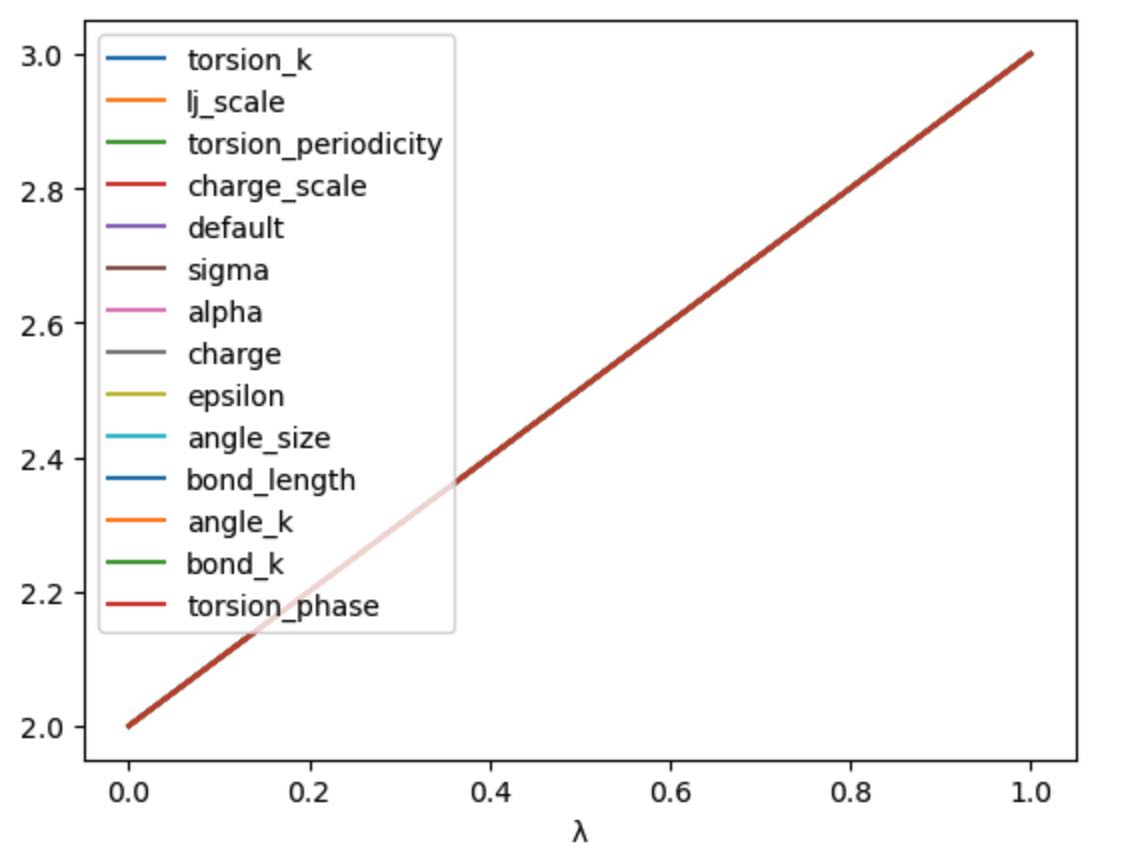
This shows how the different levers available in this schedule would morph
a hypothetical parameter that has an initial value of 2.0 and a
final value of 3.0.
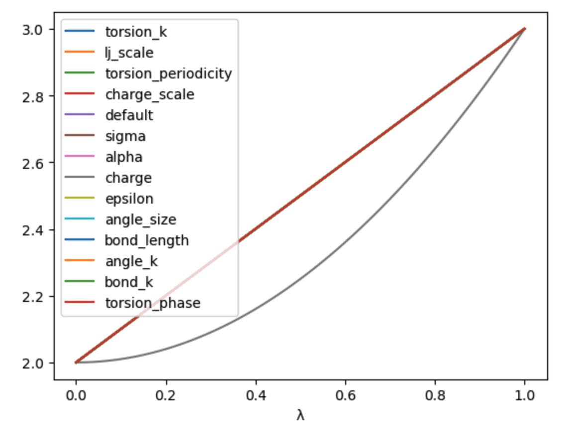
In this case the levers are all identical, so would change the parameter in the same way. You can choose your own equation for the λ-schedule. For example, maybe we want to scale the charge by the square of λ.
>>> s.set_equation(stage="morph", lever="charge",
...                equation=s.lam()**2 * s.final() + s.initial() * (1 - s.lam()**2))
>>> print(s)
LambdaSchedule(
  morph: λ * final + initial * (-λ + 1)
    charge: λ^2 * final + initial * (-λ^2 + 1)
)
This shows that in the default morph stage of this schedule, we will
scale the charge parameters by λ^2, while all other parameters (the
default) will scale using λ. We can plot the result of this using;
>>> s.get_lever_values(initial=2.0, final=3.0).plot(subplots=True)
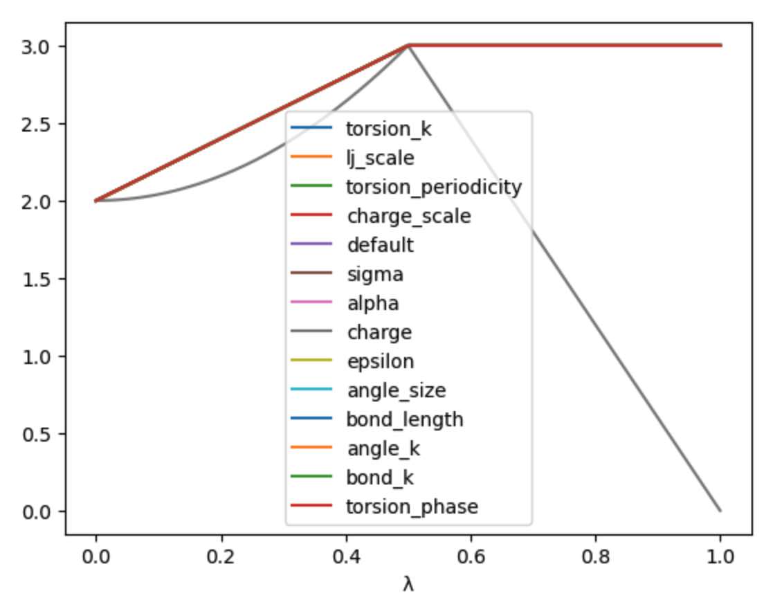
The above affected the default morph stage of the schedule. You can
append or prepend additional stages to the schedule using the
append_stage() or
prepend_stage() functions, e.g.
>>> s.append_stage("scale", s.final())
>>> print(s)
would append a second stage, called scale, which by default would
use the final value of the parameter. We could then add a lever to
this stage that scales down the charge to 0,
>>> s.set_equation(stage="scale", lever="charge",
...                equation=(1-s.lam()) * s.final())
>>> print(s)
LambdaSchedule(
  morph: λ * final + initial * (-λ + 1)
    charge: λ^2 * final + initial * (-λ^2 + 1)
  scale: final
    charge: final * (-λ + 1)
)
Again, it is worth plotting the impact of this schedule on a hypothetical parameter.
>>> s.get_lever_values(initial=2.0, final=3.0).plot(subplots=True)
Note
The value of the stage-local λ in each stage moves from 0 to 1.
This is different to the global λ, which moves from 0 to 1 evenly
over all stages. For example, in this 2-stage schedule, values of
global λ between 0 and 0.5 will be in the morph stage, while
values of global λ between 0.5 and 1 will be in the scale stage.
Within the morph stage, the local λ will move from 0 to 1
(corresponding to global λ values of 0 to 0.5), while
within the scale stage, the local λ will move from 0 to 1
(corresponding to gloabl λ values of 0.5 to 1).
Through the combination of adding stages and specifyig different equations for levers, you can have a lot of control over how the perturbable properties are morphed from the reference to the perturbed states.
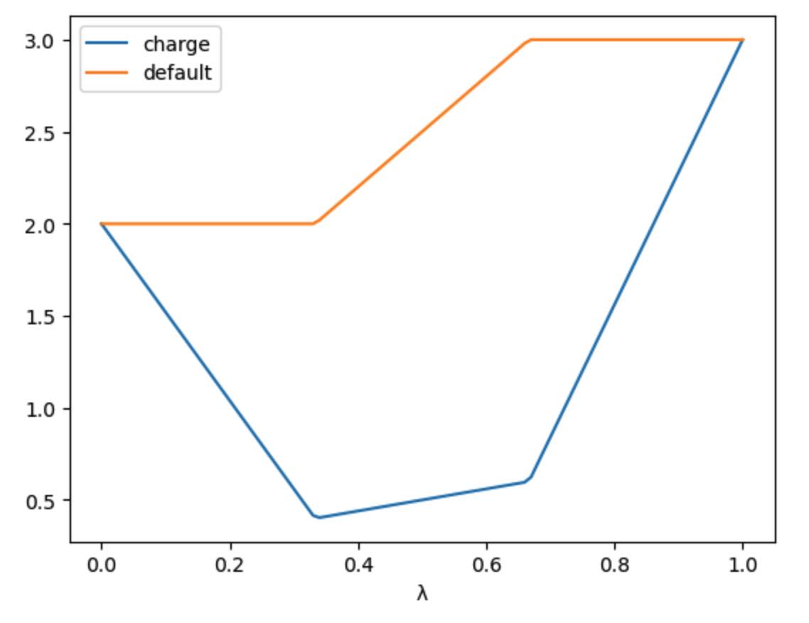
To make things easier, there are some simple functions that let you add some common stages.
>>> s = sr.cas.LambdaSchedule()
>>> print(s)
LambdaSchedule::null
>>> s.add_morph_stage("morph")
>>> print(s)
LambdaSchedule(
  morph: final * λ + initial * (-λ + 1)
)
>>> s.add_charge_scale_stages("decharge", "recharge", scale=0.2)
>>> print(s)
LambdaSchedule(
  decharge: initial
    charge: initial * (-λ * (-γ + 1) + 1)
  morph: final * λ + initial * (-λ + 1)
    charge: γ * (final * λ + initial * (-λ + 1))
  recharge: final
    charge: final * (-(-γ + 1) * (-λ + 1) + 1)
  γ == 0.2
)
has created a null schedule, and then added a morph stage using the
default perturbation equation. This is then sandwiched by two stages;
a decharge stage that scales the charge lever from the initial
value to γ times that value, and a recharge stage that scales
the charge lever from γ times the final value to the full
final value. It also scales the charge lever in the morph stage
by γ, which is set to 0.2 for all stages.
We can see how this would affect a hypothetical parameter that goes
from an initial value of 2.0 to a final value of 3.0 via
>>> s.get_lever_values(initial=2.0, final=3.0).plot(subplots=True)
Once you have created your schedule you can add it via the
set_schedule() function of the
Dynamics object, e.g.
>>> d.set_schedule(s)
Alternatively, you can set the schedule when you call the
dynamics() function, e.g.
>>> d = mols.dynamics(lambda_value=0.5, timestep="4fs", temperature="25oC",
...                   schedule=s)
>>> print(d.get_schedule())
LambdaSchedule(
  decharge: initial
    charge: (-(-γ + 1) * λ + 1) * initial
  morph: final * λ + (-λ + 1) * initial
    charge: γ * (final * λ + (-λ + 1) * initial)
  recharge: final
    charge: (-(-γ + 1) * (-λ + 1) + 1) * final
  γ == 0.2
)
Ghost Atoms and Softening potentials
Internally the alchemical dynamics simulation works by calculating morphed forcefield parameters whenever λ is changed, and then calling the OpenMM updateParametersInContext function function to update those parameters in all of the OpenMM Force objects that are used to calculate atomic forces. This is a very efficient way of performing a perturbation, as it allows vanilla (standard) OpenMM forces to be used for the dynamics. However, there are challenges with how we handle atoms which are created or deleted during the perturbation.
These atoms, which we call “ghost atoms”, provide either a space into which a new atom is grown, or a space from which an atom is deleted. To ensure these ghost atoms don’t cause dynamics instabilities, we use a softening potential to model their interactions with all other atoms. These softening potentials (also called “soft-core” potentials) soften the charge and Lennard-Jones interactions between the ghost atoms and all other atoms using an α (alpha) parameter. This is a perturbable parameter of the atoms, which is equal to 1 when the atom is in a ghost state, and 0 when it is not. For example, an atom which exists in the reference state but becomes a ghost in the perturbed state would have an α value that would go from 0 to 1. Alternatively, an atom which does not exist in the reference state, and that appears in the perturbed state, would have an α value that would go from 1 to 0.
Note
You can have as many or few ghost atoms as you want in your merged molecule. If all atoms become ghosts, then this is the same as completely decoupling the molecule, as you would do in an absolute binding free energy calculation. Equally, you could run a “dual topology” calculation by two sets of atoms in your merged molecule - the first set start as the reference state atoms, and all become ghosts, while the second set start all as ghosts and become the perturbed state atoms. In “single topology” calculations you would only use ghost atoms for those which don’t exist in either of the end states.
There are two parameters that control the softening potential:
shift_delta- set theshift_deltaparameter which is used to control the electrostatic and van der Waals softening potential that smooths the creation or deletion of ghost atoms. This is a floating point number that defaults to1.0, which should be good for most perturbations.coulomb_power- set thecoulomb_powerparameter which is used to control the electrostatic softening potential that smooths the creation and deletion of ghost atoms. This is an integer that defaults to0, which should be good for most perturbations.
Low level interface
The high-level interface is just a set of convienient wrappers around the OpenMM objects which are used to run the simulation. If you convert any set of views (or view) that contains merged molecules, then an alchemical OpenMM context will be returned.
>>> context = sr.convert.to(mols, "openmm")
>>> print(context)
openmm::Context( num_atoms=12167 integrator=VerletIntegrator timestep=1.0 fs platform=HIP )
The context is held in a low-level class,
SOMMContext, which inherits from the
standard OpenMM Context
class.
The class adds some additional metadata and control functions that are needed to update the atomic parameters in the OpenMM Context to represent the molecular system at different values of λ.
The key additional functions provided by SOMMContext
are;
get_lambda()- return the current value of λ for the context.set_lambda()- set the new value of λ for the context. Note that this should only really be used to change λ to evaluate energies at different λ-windows. It is better to re-create the context if you want to simulate at a different λ-value. This function can also be used to set therest2_scaleparameter for the context.get_lambda_schedule()- return the λ-schedule used to control the morph.set_lambda_schedule()- set the λ-schedule used to control the morph.get_energy()- return the current potential energy of the context. This will be insireunits ifto_sire_unitsisTrue(the default).
Note that you can also set the lambda_value and lambda_schedule
when you create the context using the map, e.g.
>>> context = sr.convert.to(mols, "openmm",
...                         map={"lambda_value": 0.5, "schedule": s})
>>> print(context)
openmm::Context( num_atoms=12167 integrator=VerletIntegrator timestep=1.0 fs platform=HIP )
>>> print(context.get_lambda())
0.5
>>> print(context.get_lambda_schedule())
LambdaSchedule(
  decharge: initial
    charge: (-(-γ + 1) * λ + 1) * initial
  morph: final * λ + (-λ + 1) * initial
    charge: γ * (final * λ + (-λ + 1) * initial)
  recharge: final
    charge: (-(-γ + 1) * (-λ + 1) + 1) * final
  γ == 0.2
)
You can then run dynamics as you would do normally using the standard OpenMM python API, e.g.
>>> integrator = context.getIntegrator()
>>> integrator.step(100)
You can then call get_potential_energy() and set_lambda() to
get the energy during dynamics for different values of λ, e.g.
>>> context.set_lambda(0.0)
>>> print(context.get_lambda(), context.get_potential_energy())
0.0 -38727.2 kcal mol-1
>>> context.set_lambda(0.5)
>>> print(context.get_lambda(), context.get_potential_energy())
0.5 -38743.8 kcal mol-1