Ghost Atoms and Softening Potentials

Ghost atoms are used by the sire/OpenMM interface to represent atoms that either appear or disappear during a perturbation. They are used as part of the implementation of a soft-core potential in OpenMM, to avoid singularities / crashes when atoms are annihilated or created.

A ghost atom is one which has zero charge and zero LJ parameters in either the reference or perturbed end states.

Note

In this case, “zero LJ parameters” means either the sigma or epsilon parameter is zero (or both).

Only atoms that have a zero charge and zero LJ parameters at either end state are ghost atoms. These atoms are treated differently to the rest of the atoms in the system.

All normal atoms (called “non-ghost atoms”) are treated as standard atoms in the sire to OpenMM conversion, and added to standard OpenMM Force objects (e.g. NonBondedForce, HarmonicBondForce, etc).

Ghost atoms are treated differently. They are added to the OpenMM Force objects as other atoms, but with the following key difference:

• Ghost atoms are added to the NonBondedForce with their standard charge, but with zero LJ parameters. This means that only the electrostatic energy and force from ghost atoms is evaluated here.

Ghost atoms are then added to three custom OpenMM Forces:

1. A CustomNonbondedForce called the “ghost/ghost” force. This uses a custom energy function to calculate the soft-core electrostatic and LJ interactions between all ghost atoms. It also calculates the “hard” electrostatic interaction and subtracts this from the total (to remove the real-space contribution that was calculated in the standard OpenMM NonBondedForce).

2. A CustomNonbondedForce called the “ghost/non-ghost” force. This uses a custom energy function to calculate the soft-core electrostatic and LJ interactions between all ghost atoms and all non-ghost atoms. It also calculates the “hard” electrostatic interaction and subtracts this from the total (to remove the real-space contribution that was calculated in the standard OpenMM NonBondedForce).

3. A CustomBondForce called the “ghost-14” force. This uses a custom energy function to calculate the soft-core electrostatic and LJ interactions between all 1-4 non-bonded interactions involving ghost atoms. It also calculates the “hard” electrostatic interaction and subtracts this from the total (to remove the real-space contribution that was calculated in the standard OpenMM NonBondedForce).

There are two different soft-core potentials available. The default is the Zacharias potential, while the second is the Taylor potential.

Zacharias softening

This is the default soft-core potential. You can also use it by setting the map option use_zacharias_softening to True.

It is based on the following electrostatic and Lennard-Jones potentials:

\[ \begin{align}\begin{aligned}V_{\text{elec}}(r) = q_i q_j \left[ \frac{(1 - \alpha)^n}{\sqrt{r^2 + \delta_\text{coulomb}^2}} - \frac{\kappa}{r} \right]\\V_{\text{LJ}}(r) = 4\epsilon \left[ \frac{\sigma^{12}}{(\delta_\text{LJ} \sigma + r^2)^6} - \frac{\sigma^6}{(\delta_\text{LJ} \sigma + r^2)^3} \right]\end{aligned}\end{align} \]

where

\[ \begin{align}\begin{aligned}\delta_\text{coulomb} = \alpha \times \text{shift_coulomb}\\\delta_\text{LJ} = \alpha \times \text{shift_LJ}\end{aligned}\end{align} \]

and

\[ \begin{align}\begin{aligned}\alpha = \max(\alpha_i, \alpha_j)\\\kappa = \max(\kappa_i, \kappa_j)\end{aligned}\end{align} \]

The parameters r, q_i, q_j, \epsilon, and \sigma are the standard parameters for the electrostatic and Lennard-Jones potentials.

The soft-core parameters are:

• α_i and α_j control the amount of “softening” of the electrostatic and LJ interactions. A value of 0 means no softening (fully hard), while a value of 1 means fully soft. Ghost atoms which disappear as a function of λ have a value of α of 1 in the reference state, and 0 in the perturbed state. Ghost atoms which appear as a function of λ have a value of α of 0 in the reference state, and 1 in the perturbed state. These values can be perturbed via the alpha lever in the λ-schedule.

• n is the “coulomb power”, and is set to 0 by default. It can be any integer between 0 and 4. It is set via coulomb_power map parameter.

• shift_coulomb and shift_LJ are the so-called “shift delta” parameters, which are specified individually for the coulomb and LJpotentials. They are set via the shift_coulomb and shift_delta map parameters. They default to 1 Å and 2.5 Å respectively.

• κ_i and κ_j are the “hard” electrostatic parameters, which control whether or not to calculate the “hard” electrostatic interaction to subtract from the total energy and force (thus cancelling out the double-counting of this interaction from the NonbondedForce). By default, these are always equal to 1. You can perturb these via the kappa lever in the λ-schedule, e.g. if you want to decouple the intramolecular electrostatic interactions, when the “hard” interaction would not be calculated in the NonbondedForce.

Taylor softening

This is the second soft-core potential. You can use it by setting the map option use_taylor_softening to True.

It is based on the following electrostatic and Lennard-Jones potentials:

\[ \begin{align}\begin{aligned}V_{\text{elec}}(r) = q_i q_j \left[ \frac{(1 - \alpha)^n}{\sqrt{r^2 + \delta^2}} - \frac{\kappa}{r} \right]\\V_{\text{LJ}}(r) = 4\epsilon \left[ \frac{\sigma^{12}}{(\alpha^m \sigma^6 + r^6)^2} - \frac{\sigma^6}{\alpha^m \sigma^6 + r^6} \right]\end{aligned}\end{align} \]

where

\[\delta = \alpha \times \text{shift_coulomb}\]

and

\[ \begin{align}\begin{aligned}\alpha = \max(\alpha_i, \alpha_j)\\\kappa = \max(\kappa_i, \kappa_j)\end{aligned}\end{align} \]

The parameters r, q_i, q_j, \epsilon, and \sigma are the standard parameters for the electrostatic and Lennard-Jones potentials.

The soft-core parameters are:

• α_i and α_j control the amount of “softening” of the electrostatic and LJ interactions. A value of 0 means no softening (fully hard), while a value of 1 means fully soft. Ghost atoms which disappear as a function of λ have a value of α of 1 in the reference state, and 0 in the perturbed state. Ghost atoms which appear as a function of λ have a value of α of 0 in the reference state, and 1 in the perturbed state. These values can be perturbed via the alpha lever in the λ-schedule.

• m is the “taylor power”, and is set to 1 by default. It can be any integer between 0 and 4. It is set via taylor_power map parameter.

• n is the “coulomb power”, and is set to 0 by default. It can be any integer between 0 and 4. It is set via coulomb_power map parameter.

• shift_coulomb is the so-called “shift delta” parameters, which are specified only for the coulomb potential. This is set via the shift_coulomb map parameters. This defaults to 1 Å.

• κ_i and κ_j are the “hard” electrostatic parameters, which control whether or not to calculate the “hard” electrostatic interaction to subtract from the total energy and force (thus cancelling out the double-counting of this interaction from the NonbondedForce). By default, these are always equal to 1. You can perturb these via the kappa lever in the λ-schedule, e.g. if you want to decouple the intramolecular electrostatic interactions, when the “hard” interaction would not be calculated in the NonbondedForce.

Good practice

Softening potentials can help to avoid singularities and crashes when atoms are annihilated or created. However, you still need to be careful when using them. For example, it is best when creating or destroying an atom to keep the sigma LJ parameter the same for both end states. This way, only the epsilon parameter is scaled to zero, while the atom keeps its same “size”. This avoids the atom shrinking as a function of λ, which could result in atoms (and thus charges) getting too close to one another.

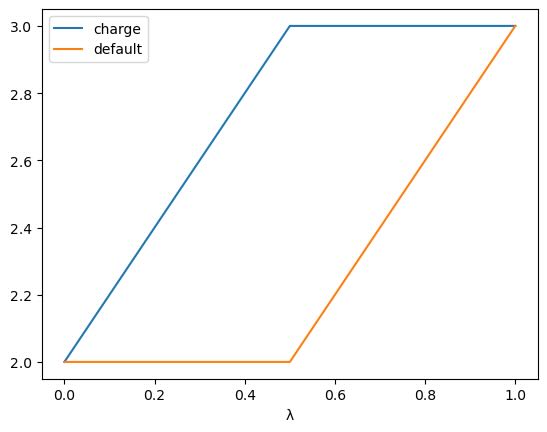
For complex or large molecules, it may be better to separate out the decharging from the decoupling or annihilation, e.g. first set up a λ-schedule to have two stages; the first stage decouples the charges, while the second stage annihilates or decouples the atoms.

This could be achieved using the following λ-schedule:

>>> import sire as sr
>>> s = sr.cas.LambdaSchedule.standard_morph()
>>> s.set_equation(stage="morph", lever="charge", equation=s.final())
>>> s.prepend_stage("decharge", s.initial())
>>> s.set_equation(stage="decharge", lever="charge",
...                equation=l.lam() * s.final() + s.initial() * (1 - s.lam()))
>>> s.get_lever_values(initial=2.0, final=3.0).plot()