Alchemical Restraints#

You can perturb restraints as part of an alchemical free energy simulation. This is useful for computing free energy differences between two systems where you want to turn on or off restraints that are used to keep part of the molecules in place while you are performing the mutation.

You can perturb restraints by adding them to the LambdaSchedule used to control the perturbation.

By default, restraints are called restraint, and so are perturbed using the restraint lever.

>>> import sire as sr
>>> l = sr.cas.LambdaSchedule()
>>> l.add_stage("restraints_on", l.initial())
>>> l.add_stage("morph", (1-l.lam()) * l.initial() + l.lam() * l.final())
>>> l.add_stage("restraints_off", l.final())
>>> print(l)
LambdaSchedule(
  restraints_on: initial
  morph: initial * (-λ + 1) + λ * final
  restraints_off: final
)

This has created a schedule with three stages, restraints_on, morph and restraints_off. The morph stage is the one that will be used to peturb the molecule from the initial state to the perturbed state.

The restraints_on and restraints_off stages will be used to switch on and off the restraints. To actually switch them on and off, we need to set the equation that will be used to scale the restraints.

>>> l.set_equation("restraints_on", "restraint", l.lam() * l.initial())
>>> l.set_equation("restraints_off", "restraint", (1-l.lam()) * l.initial())

This will scale the restraints by λ in the restraints_on stage. This means that the restraints start at λ=0 scaled to 0, and are then fully switched on by λ=1.

The restraints are scaled off by (1-λ) in the restraints_off stage. This means that the restraints are fully switched on at λ=0, but then scaled down so that they are scaled to 0 at λ=1.

The value of initial and final for a restraint is the same, being 100% of the restraint. Thus (1-l.lam()) * l.initial() + l.lam() * l.final() will always evaluate to 100% of the restraint for all values of λ during the morph stage. You can make sure that the restraint is kept at 100% during this stage by setting this value explicitly;

>>> l.set_equation(stage="morph", lever="restraint", l.initial())
>>> print(l)
LambdaSchedule(
  restraints_on: initial
    restraint: λ * initial
  morph: initial * (-λ + 1) + λ * final
    restraint: initial
  restraints_off: final
    restraint: final * (-λ + 1)
)

You can view the effect of this schedule by plotting the perturbation assuming an initial value of 1.0 and a final value of 2.0 using

>>> l.get_lever_values(initial=1.0, final=2.0).plot()

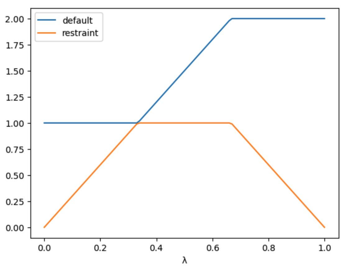
Impact of the schedule on parameters from 1.0 to 2.0

Here we can see the three stages of the schedule. The restraints_on stage keeps the default value of the restraint at the initial value (1.0) while it scales the restraint from 0 to 1.0. The morph stage keeps the restraint at 1.0, while scaling the parameter from 1.0 to 2.0. Finally, the restraints_off stage scales the restraint from 1.0 to 0 while keeping the parameter at 2.0.

We can now use this schedule to perturb the restraints during an alchemical simulation e.g.

>>> mols = sr.load(sr.expand(sr.tutorial_url, "merged_molecule.s3"))
>>> restraints = sr.restraints.positional(mols, "molidx 0")
>>> mols = mols.minimisation(restraints=restraints,
...                          lambda_value=0.0).run().commit()
>>> d = mols.dynamics(timestep="4fs", temperature="25oC",
...                   restraints=restraints, schedule=l,
...                   lambda_value=0.0)
>>> d.run("10ps")
>>> mols = d.commit()

Using named restraints#

By default, all restraints in a system are called restraint, and so are perturbed using the restraint lever. However, you can also give restraints their own name, and then perturb them using their name. For example, here we create two restraints, named positional and distance.

>>> pos_rest = sr.restraints.positional(mols, "molidx 0", name="positional")
>>> dst_rest = sr.restraints.distance(mols, atoms0=0, atoms1=1, name="distance")
>>> print(pos_rest, dst_rest)
PositionalRestraints( name=positional, size=8
0: PositionalRestraint( 0 => ( 25.7128, 24.9375, 25.2539 ), k=150 kcal mol-1 Å-2 : r0=0 Å )
1: PositionalRestraint( 1 => ( 24.2872, 25.0626, 24.7461 ), k=150 kcal mol-1 Å-2 : r0=0 Å )
2: PositionalRestraint( 2 => ( 25.9115, 23.8899, 25.5639 ), k=150 kcal mol-1 Å-2 : r0=0 Å )
3: PositionalRestraint( 3 => ( 26.425, 25.2206, 24.4509 ), k=150 kcal mol-1 Å-2 : r0=0 Å )
4: PositionalRestraint( 4 => ( 25.8616, 25.6094, 26.1259 ), k=150 kcal mol-1 Å-2 : r0=0 Å )
5: PositionalRestraint( 5 => ( 24.1384, 24.3907, 23.8741 ), k=150 kcal mol-1 Å-2 : r0=0 Å )
6: PositionalRestraint( 6 => ( 24.0888, 26.1101, 24.4351 ), k=150 kcal mol-1 Å-2 : r0=0 Å )
7: PositionalRestraint( 7 => ( 23.575, 24.7795, 25.5491 ), k=150 kcal mol-1 Å-2 : r0=0 Å )
) BondRestraints( name=distance, size=1
0: BondRestraint( 0 <=> 1, k=150 kcal mol-1 Å-2 : r0=1.5185 Å )
)

We can now create a schedule that perturbs these restraints separately using their names. We will first scale up the distance restraint in a distance_restraints stage…

>>> l = sr.cas.LambdaSchedule()
>>> l.add_stage("distance_restraints", 0)
>>> l.set_equation(stage="distance_restraints", lever="distance",
...                equation=l.lam() * l.initial())

and will then scale up the positional restraint in a positional_restraints stage, while keeping the distance restraint fully on.

>>> l.add_stage("positional_restraints", 1)
>>> l.set_equation(stage="positional_restraints", lever="positional",
...                equation=l.lam() * l.initial())
>>> print(l)
LambdaSchedule(
  distance_restraints: 0
    distance: λ * initial
  positional_restraints: 1
    positional: λ * initial
)
>>> l.get_lever_values(initial=1.0, final=1.0,
...                    levers=["positional", "distance"]).plot()

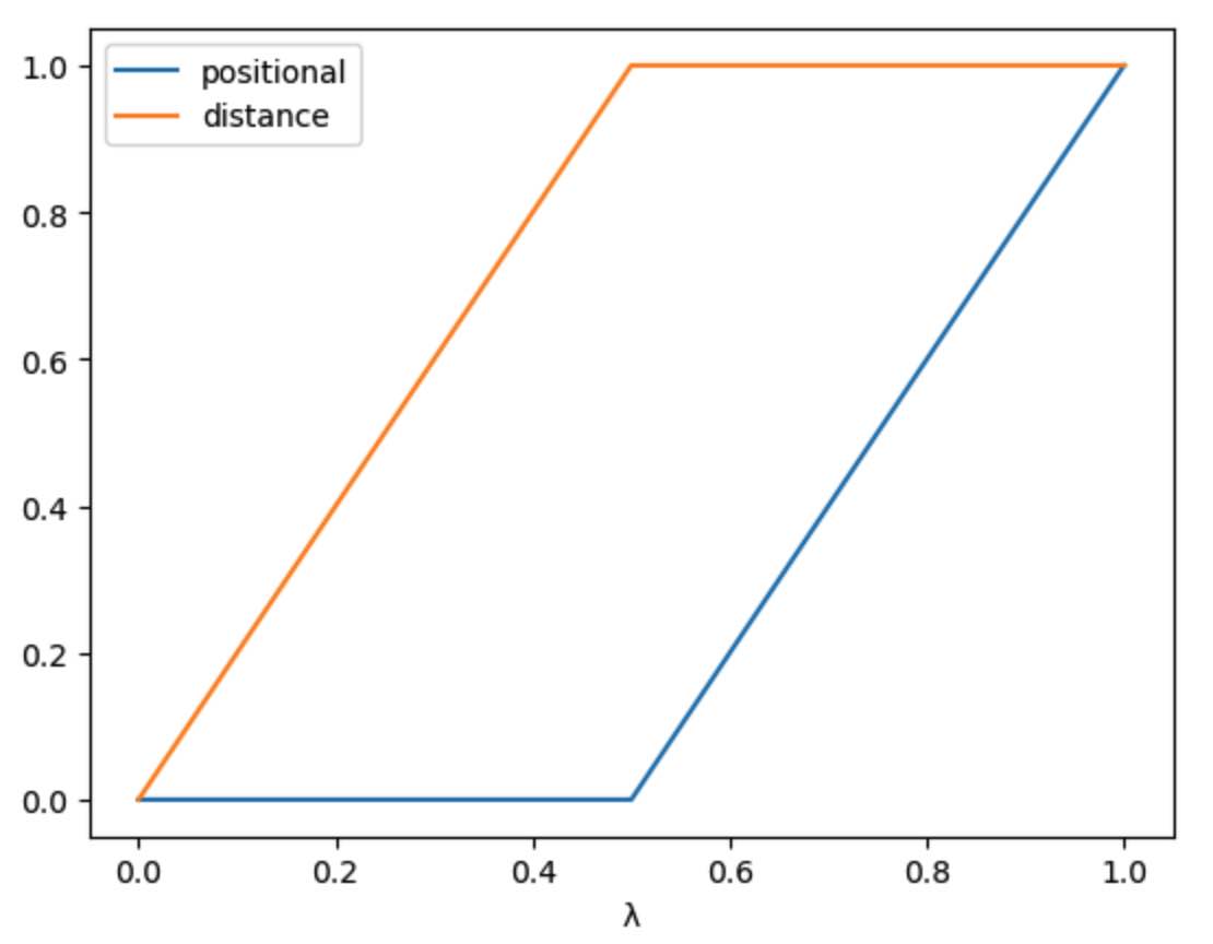
Impact of the schedule for scaling two restraints separately

Here we can see that, in the first distance_restraints stage (from λ=0 to λ=0.5), the distance restraint is scaled from 0 to 1 while the positional restraint is kept at 0. In the second positional_restraints stage (from λ=0.5 to λ=1), the positional restraint is scaled from 0 to 1 while the distance restraint is kept at 1.

We can now use this schedule in a simulation, e.g.

>>> mols = sr.load(sr.expand(sr.tutorial_url, "merged_molecule.s3"))
>>> mols = mols.minimisation(restraints=[dst_rest, pos_rest],
...                          lambda_value=0.0).run().commit()
>>> d = mols.dynamics(timestep="4fs", temperature="25oC",
...                   restraints=[dst_rest, pos_rest], schedule=l,
...                   lambda_value=0.0)
>>> d.run("10ps")
>>> mols = d.commit()