Perturbation
As seen in chapter 6, the concept of a
“merged molecule” is central to how sire implements the
perturbations (morphing) needed for free energy calculations.
A merged molecule is one that has been created with a single set of atoms, but with properties that represent either a “reference” (λ=0) or “perturbed” (λ=1) state.
For example, let’s load a merged molecule that represents neopentane in the reference state, and methane in the perturbed state.
>>> import sire as sr
>>> mols = sr.load_test_files("neo_meth_scratch.bss")
>>> print(mols)
System( name=BioSimSpace_System num_molecules=1 num_residues=1 num_atoms=17 )
>>> print(mols[0])
Molecule( Merged_Molecule:6 num_atoms=17 num_residues=1 )
Note
This molecule was created using BioSimSpace. We will cover how to create merged molecules in a later section in this tutorial.
Examining the perturbation
Normally, a sire molecule will have one set of forcefield parameters.
For example, the atomic charges would be stored in the charge property,
the Lennard-Jones parameters in the LJ property, the bond parameters in
the bond property, etc.
However, a merged molecule has two sets of parameters, one for the reference
state (representing λ=0) and one for the perturbed state (representing λ=1).
The reference state parameters are stored in the 0 properties, e.g.
charge0, LJ0, bond0, etc. The perturbed state parameters are
stored in the 1 properties, e.g. charge1, LJ1, bond1, etc.
We can see this for our merged molecule above by printing out all of the property keys.
>>> print(mols[0].property_keys())
['gb_radii0', 'gb_radii1', 'atomtype0', 'element0', 'atomtype1', 'element1',
 'time', 'intrascale0', 'intrascale1', 'improper0', 'mass0', 'improper1',
 'mass1', 'ambertype0', 'ambertype1', 'treechain0', 'treechain1',
 'parameters0', 'parameters1', 'space', 'charge0', 'charge1',
 'connectivity', 'dihedral0', 'forcefield0', 'dihedral1', 'coordinates0',
 'forcefield1', 'coordinates1', 'LJ0', 'name0', 'LJ1', 'name1', 'angle0',
 'angle1', 'bond0', 'bond1', 'molecule0', 'molecule1', 'gb_screening0',
 'gb_screening1', 'is_perturbable']
Notice how there is a 0 and 1 version of nearly every property.
These represent the molecule at the reference and perturbed end states, e.g.
>>> print(mols[0].property("charge0"))
SireMol::AtomCharges( size=17
0: -0.0853353 |e|
1: -0.0602353 |e|
2: -0.0853353 |e|
3: -0.0853353 |e|
4: -0.0853353 |e|
...
12: 0.0334647 |e|
13: 0.0334647 |e|
14: 0.0334647 |e|
15: 0.0334647 |e|
16: 0.0334647 |e|
)
>>> print(mols[0].property("charge1"))
SireMol::AtomCharges( size=17
0: 0 |e|
1: 0.0271 |e|
2: 0 |e|
3: -0.1084 |e|
4: 0 |e|
...
12: 0.0271 |e|
13: 0.0271 |e|
14: 0 |e|
15: 0 |e|
16: 0 |e|
)
prints the charges for neopentane, and then methane. Note how many of the
atom charges for methane are zero. This is because methane has fewer
atoms than neopentane, and so the charges (and other parameters) for the
extra atoms are “switched off” for the perturbed state. These extra atoms
are often called “dummy atoms”. In sire, we prefer to call them
“ghost atoms”. They are “ghosts” because they fade away to nothing as
λ increases from 0 to 1.
In addition to the 0 and 1 properties, a perturbable molecule must
also contain the is_perturbable property. This is a boolean that signals
whether or not a molecule is perturbable. It should be True if the molecule
can be perturbed.
>>> print(mols[0].property("is_perturbable"))
True
Perturbation objects
Examining the perturbable properties directly can be a little cumbersome.
To make things easier, there are a number of helper classes and functions.
These are accessed via the sire.morph module, and the
perturbation() function of a Molecule.
Let’s create the Perturbation object for our molecule.
>>> pert = mols[0].perturbation()
>>> print(pert)
Perturbation( Molecule( Merged_Molecule:6 num_atoms=17 num_residues=1 ) )
We can extract a molecule that contains only the reference or perturbed
parameters using the extract_reference() and
extract_perturbed() functions.
>>> ref = pert.extract_reference()
>>> print(ref.property_keys())
['bond', 'atomtype', 'time', 'intrascale', 'element', 'dihedral',
 'parameters', 'ambertype', 'angle', 'gb_radii', 'treechain', 'space',
 'forcefield', 'name', 'connectivity', 'gb_screening', 'molecule',
 'coordinates', 'LJ', 'charge', 'mass', 'improper']
>>> print(ref.property("charge"))
SireMol::AtomCharges( size=17
0: -0.0853353 |e|
1: -0.0602353 |e|
2: -0.0853353 |e|
3: -0.0853353 |e|
4: -0.0853353 |e|
...
12: 0.0334647 |e|
13: 0.0334647 |e|
14: 0.0334647 |e|
15: 0.0334647 |e|
16: 0.0334647 |e|
)
Note
You can extract the reference and perturbed molecules in a collection
using the sire.morph.extract_reference() and
sire.morph.extract_perturbed() functions. For example,
mols = sire.morph.extract_reference(mols) would extract the
reference state of all molecules in mols.
Note
By default, ghost atoms will be removed when you extract an end state.
You can retain ghost atoms by passing remove_ghosts=False to the
above extract_reference and extract_perturbed functions.
Extracting the reference or perturbed states can be useful if you want to
go back to the unmerged molecule, e.g. for visualisation via the
view() function. However, normally we would want to
keep the properties of the two end states, and then choose one end state
as the “current” state. We can do this by creating links from the
“standard” property names (e.g. charge, LJ etc.) to the equivalent
properties of the chosen end state. You could do this manually, but it is
much easier to use the link_to_reference()
and link_to_perturbed() functions.
For example, here we will link to the perturbed state.
>>> mol = pert.link_to_perturbed()
>>> print(mol.get_links())
{'improper': 'improper1', 'gb_screening': 'gb_screening1',
 'mass': 'mass1', 'dihedral': 'dihedral1', 'parameters': 'parameters1',
 'treechain': 'treechain1', 'bond': 'bond1', 'ambertype': 'ambertype1',
 'molecule': 'molecule1', 'atomtype': 'atomtype1', 'charge': 'charge1',
 'angle': 'angle1', 'forcefield': 'forcefield1',
 'coordinates': 'coordinates1', 'intrascale': 'intrascale1',
 'name': 'name1', 'LJ': 'LJ1', 'element': 'element1',
 'gb_radii': 'gb_radii1'}
>>> print(mol.property("charge"))
SireMol::AtomCharges( size=17
0: 0 |e|
1: 0.0271 |e|
2: 0 |e|
3: -0.1084 |e|
4: 0 |e|
...
12: 0.0271 |e|
13: 0.0271 |e|
14: 0 |e|
15: 0 |e|
16: 0 |e|
)
Note
You can link the reference or perturbed states in a collection of
molecules using the sire.morph.link_to_reference() and
sire.morph.link_to_perturbed() functions. For example,
mols = sire.morph.link_to_perturbed(mols) would link all molecules
in mols to the perturbed state.
Note
It is a good idea when loading a system containing one or more merged
molecules to decide on which end state you want to use as the “current”.
After loading, simply call either
mols = sire.morph.link_to_reference(mols) or
mols = sire.morph.link_to_perturbed(mols) to update the molecules
with your chosen state.
Inspecting the changing parameters
Under the hood, the properties of the two end states are converted into
parameters for the underlying OpenMM system used for the
free energy simulations. You can access these parameters by converting
the above perturbation into a
PerturbableOpenMMMolecule.
>>> pert_omm = pert.to_openmm()
>>> print(pert_omm)
PerturbableOpenMMMolecule()
This object contains all of the parameters needed to represent both
end states of this molecule in the OpenMM forces. For example,
get_charges0()
returns a list of the charges for the reference
state, while
get_charges0()
returns a list of the charges for the perturbed state.
>>> print(pert_omm.get_charges0())
[-0.08533529411764705, -0.06023529411764705, -0.08533529411764705,
 -0.08533529411764705, -0.08533529411764705, 0.03346470588235294,
  0.03346470588235294, 0.03346470588235294, 0.03346470588235294,
  0.03346470588235294, 0.03346470588235294, 0.03346470588235294,
  0.03346470588235294, 0.03346470588235294, 0.03346470588235294,
  0.03346470588235294, 0.03346470588235294]
At this level, we are most interested in the parameters that change as
we morph from the reference to the perturbed state (i.e. as we move
from λ=0 to λ=1). You can access these via the
changed_atoms(),
changed_bonds(),
changed_angles(),
changed_torsions(),
changed_exceptions() and
changed_constraints()
functions.
>>> print(pert_omm.changed_bonds())
        bond  length0  length1         k0         k1
0  C2:2-C4:4  0.15375  0.10969  251793.12  276646.08
>>> print(pert_omm.changed_angles())
              angle     size0     size1        k0        k1
0  C2:2-C4:4-H12:12  1.916372  1.877626  387.4384  329.6992
1  C2:2-C4:4-H14:14  1.916372  1.877626  387.4384  329.6992
2  C2:2-C4:4-H13:13  1.916372  1.877626  387.4384  329.6992
Note
The parameters are directly as would be used in an OpenMM force, i.e. in OpenMM default units.
Here we see that the perturbation involves the C2-C4 bond changing from 0.15375 nm to 0.10969 nm, with an associated change in the force constant from 251793.12 kJ mol^-1 nm^-2 to 276646.08 kJ mol^-1 nm^-2.
Similarly, the C2-C4-H12 angle changes from 1.916372 radians to 1.877626 radians, with an associated change in the force constant from 387.4384 kJ mol^-1 rad^-2 to 329.6992 kJ mol^-1 rad^-2.
These functions return their output as pandas dataframes. You can get a raw
output by passing in to_pandas=False.
>>> print(pert_omm.changed_bonds(to_pandas=False))
[(Bond( C2:2 => C4:4 ), 0.15375000000000003, 0.10969000000000001, 251793.11999999997, 276646.08)]
As well as forcefield parameters, you can also access any changes in
constraint parameters caused by constraining perturbable bonds. For example,
here we can create the PerturbableOpenMMMolecule
used when the bonds constraint algorithm is used.
>>> pert_omm = pert.to_openmm(constraint="bonds")
Now, we can see how the constraint parameters will change across λ using
the changed_constraints()
function.
>>> print(pert_omm.changed_constraints())
    atompair  length0  length1
0  C2:2-C4:4  0.15375  0.10969
In this case, we see that the perturbing C2-C4 bond is constrained, with a constraint length of 0.15375 nm in the reference state, and 0.10969 nm in the perturbed state.
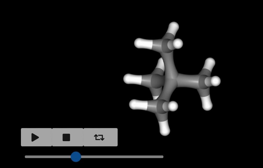
Visualising the perturbation
Perturbations can involve changes in bond lengths, or angle / torsion sizes.
These can be difficult to visualise from the raw numbers. To help with this,
the view_reference() and
view_perturbed() functions can be used to
view a 3D movie of the perturbation from either the reference or perturbed
states.
>>> pert.view_reference()
Note
The movie loops from λ=0 to λ=1, and then back to λ=0. You can pass in
any of the visualisation options as used in the standard
view() function. The viewer may show some
bonds as broken - this is just because they are too long to be shown
when calculated at λ=0.