Quick Start Guide
Import sire using
>>> import sire as sr
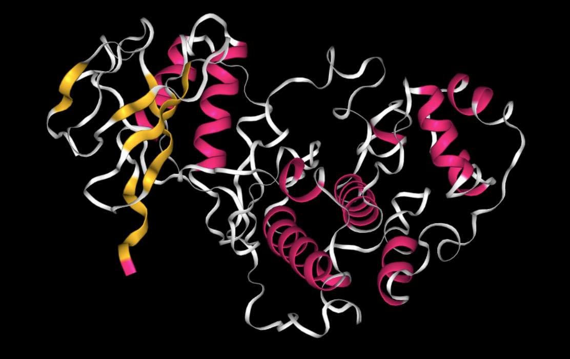
Load a molecule from a URL, via sire.load().
>>> mols = sr.load(f"{sr.tutorial_url}/p38.pdb")
Note
sire.tutorial_url expands to the base URL that contains
all tutorial files.
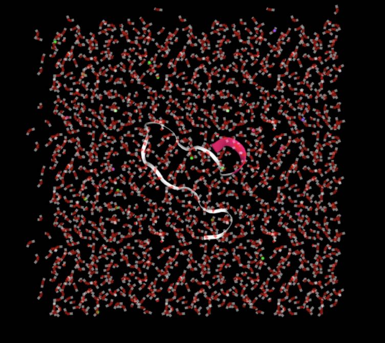
View molecules using view().
>>> mols.view()
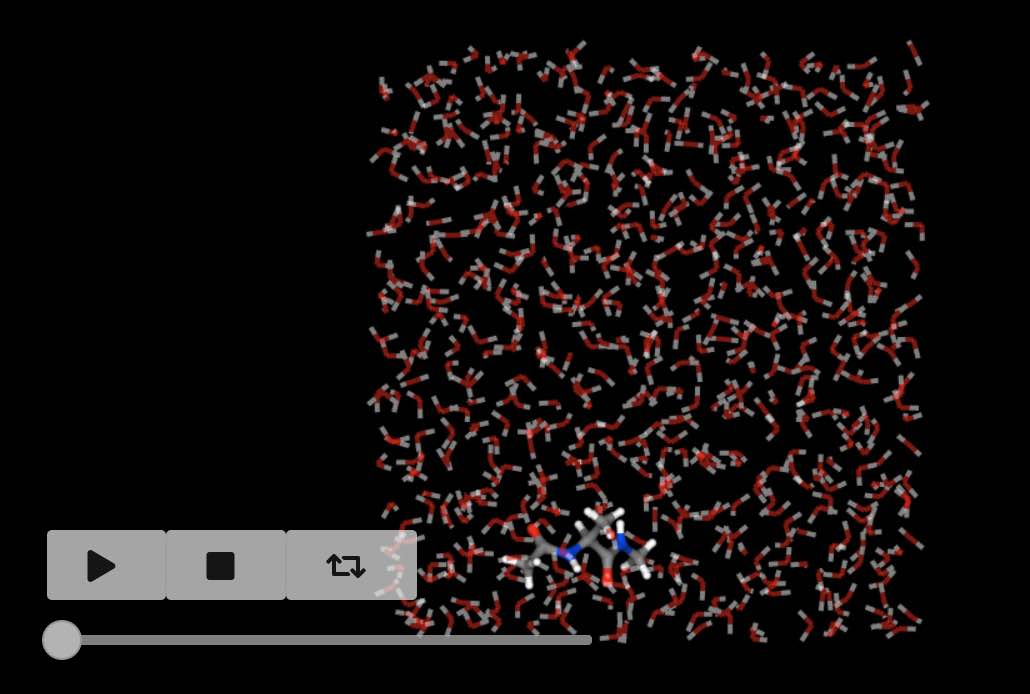
Or load molecules that need multiple input files by passing in multiple files.
>>> mols = sr.load(f"{sr.tutorial_url}/ala.top", f"{sr.tutorial_url}/ala.traj")
Note
You could use sire.expand() to put sire.tutorial_url in front
of ala.top and ala.crd, e.g. via
sr.expand(sr.tutorial_url, ["ala.top", "ala.traj"])
There are lots of ways to search or index for molecules, e.g.
>>> mols[0]
Molecule( ACE:7   num_atoms=22 num_residues=3 )
has returned the first molecule in the system of molecules that were loaded.
>>> mols["water"]
SelectorMol( size=630
0: Molecule( WAT:4   num_atoms=3 num_residues=1 )
1: Molecule( WAT:5   num_atoms=3 num_residues=1 )
2: Molecule( WAT:6   num_atoms=3 num_residues=1 )
3: Molecule( WAT:7   num_atoms=3 num_residues=1 )
4: Molecule( WAT:8   num_atoms=3 num_residues=1 )
...
625: Molecule( WAT:629 num_atoms=3 num_residues=1 )
626: Molecule( WAT:630 num_atoms=3 num_residues=1 )
627: Molecule( WAT:631 num_atoms=3 num_residues=1 )
628: Molecule( WAT:632 num_atoms=3 num_residues=1 )
629: Molecule( WAT:633 num_atoms=3 num_residues=1 )
)
has returned all of the water molecules,
while
>>> mols[0]["element C"]
Selector<SireMol::Atom>( size=6
0:  Atom( CH3:2   [  18.98,    3.45,   13.39] )
1:  Atom( C:5     [  18.48,    4.55,   14.35] )
2:  Atom( CA:9    [  16.54,    5.03,   15.81] )
3:  Atom( CB:11   [  16.05,    6.39,   15.26] )
4:  Atom( C:15    [  15.37,    4.19,   16.43] )
5:  Atom( CH3:19  [  13.83,    3.94,   18.35] )
)
has returned all of the carbon atoms in the first molecule.
Smarts searchs are supported too! For example, here are three matches for a smarts string that finds aliphatic carbons.
>>> mols["smarts [#6]!:[#6]"]
AtomMatch( size=3
0: [2] CH3:2,C:5
1: [2] CA:9,CB:11
2: [2] CA:9,C:15
)
You can also search for bonds, e.g.
>>> mols[0].bonds()
SelectorBond( size=21
0: Bond( HH31:1 => CH3:2 )
1: Bond( CH3:2 => HH32:3 )
2: Bond( CH3:2 => HH33:4 )
3: Bond( CH3:2 => C:5 )
4: Bond( C:5 => O:6 )
...
16: Bond( N:17 => H:18 )
17: Bond( N:17 => CH3:19 )
18: Bond( CH3:19 => HH31:20 )
19: Bond( CH3:19 => HH32:21 )
20: Bond( CH3:19 => HH33:22 )
)
has returned all of the bonds in the first molecule, while
>>> mols.bonds("element O", "element H")
SelectorMBond( size=1260
0: MolNum(4) Bond( O:23 => H1:24 )
1: MolNum(4) Bond( O:23 => H2:25 )
2: MolNum(5) Bond( O:26 => H1:27 )
3: MolNum(5) Bond( O:26 => H2:28 )
4: MolNum(6) Bond( O:29 => H1:30 )
...
1255: MolNum(631) Bond( O:1904 => H2:1906 )
1256: MolNum(632) Bond( O:1907 => H1:1908 )
1257: MolNum(632) Bond( O:1907 => H2:1909 )
1258: MolNum(633) Bond( O:1910 => H1:1911 )
1259: MolNum(633) Bond( O:1910 => H2:1912 )
)
has returned all of the oxygen-hydrogen bonds in all molecules.
If a trajectory has been loaded (as is the case here) then you can get the number of frames using
>>> mols.num_frames()
500
and can view the movie using
>>> mols.view()
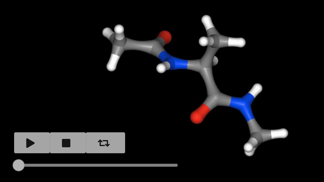
The view() function can be called on any
selection, so you can view the movie of the first molecule using
>>> mols[0].view()
You can extract a subset of trajectory frames by indexing, e.g.
>>> mols[0].trajectory()[0::100].view()
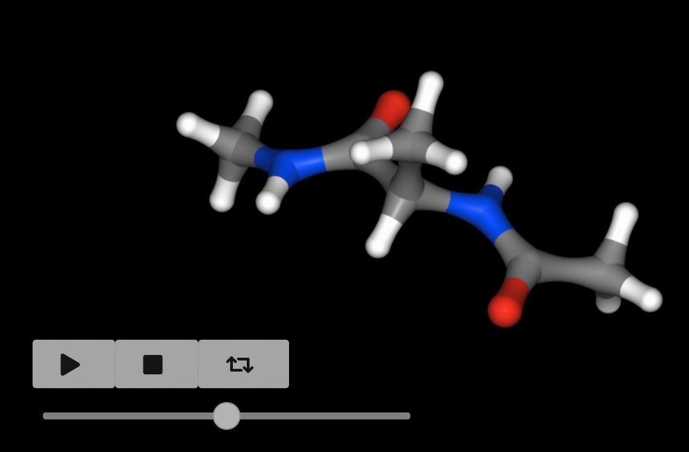
views every 100 frames of the trajectory.
If the molecule was loaded with forcefield parameters, then you can
calculate its energy using the energy()
function.
>>> mols[0].energy()
31.5691 kcal mol-1
You can get all of the components via
>>> mols[0].energy().components()
{'bond': 4.22497 kcal mol-1,
 '1-4_LJ': 3.50984 kcal mol-1,
 'angle': 7.57006 kcal mol-1,
 'dihedral': 9.80034 kcal mol-1,
 '1-4_coulomb': 44.8105 kcal mol-1,
 'intra_LJ': -1.31125 kcal mol-1,
 'improper': 0.485545 kcal mol-1,
 'intra_coulomb': -37.5208 kcal mol-1}
You can calculate the energy across a trajectory, with the results returned as a pandas dataframe!
>>> mols[0].trajectory().energy()
     frame        time    1-4_LJ  1-4_coulomb      angle      bond   dihedral  improper  intra_LJ  intra_coulomb      total
0        0    0.200000  3.509838    44.810452   7.570059  4.224970   9.800343  0.485545 -1.311255     -37.520806  31.569147
1        1    0.400000  2.700506    47.698455  12.470519  2.785874  11.776295  1.131481 -1.617496     -40.126219  36.819417
2        2    0.600000  2.801076    43.486411  11.607753  2.023439  11.614774  0.124729 -1.103966     -36.633297  33.920920
3        3    0.800000  3.365638    47.483966   6.524609  0.663454  11.383852  0.339333 -0.983872     -40.197920  28.579061
4        4    1.000000  3.534830    48.596027   6.517530  2.190370  10.214994  0.255331 -1.699613     -40.355054  29.254415
..     ...         ...       ...          ...        ...       ...        ...       ...       ...            ...        ...
495    495   99.199997  2.665994    42.866319  11.339087  4.172684   9.875872  0.356887 -1.584092     -36.499764  33.192988
496    496   99.400002  3.062467    44.852774   9.268408  1.878366  10.548897  0.327064 -1.814718     -36.671683  31.451575
497    497   99.599998  3.530233    44.908117  10.487378  4.454670  10.223964  1.006034 -0.692972     -37.118048  36.799376
498    498   99.800003  3.511116    42.976288   9.017446  0.809064  10.841436  0.518190 -1.862433     -35.481467  30.329641
499    499  100.000000  3.768998    41.625135  13.629923  1.089916  11.889372  0.846805 -1.897328     -36.547672  34.405149
You can do more with the molecule, for example viewing it’s 2D structure
>>> mols[0].view2d()
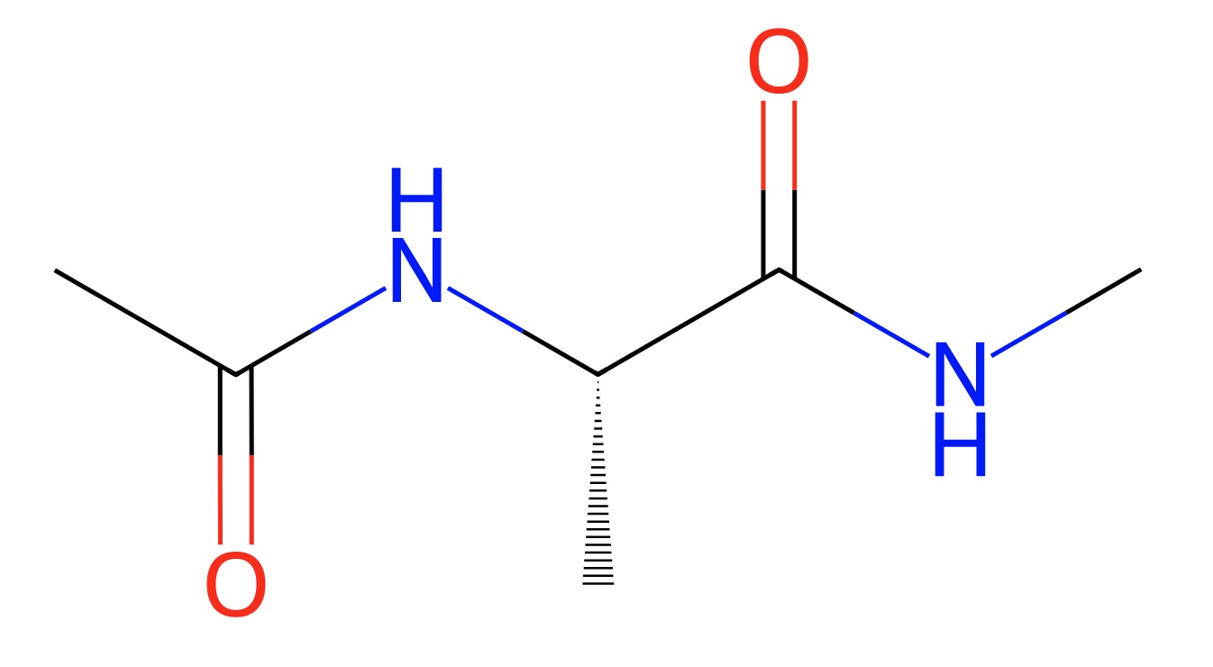
or generating its smiles string.
>>> mols[0].smiles()
'CNC(=O)C(C)NC(C)=O'
You can also convert it to an RDKit molecule!
>>> rdmol = sr.convert.to(mols[0], "rdkit")
And you can even run molecular dynamics using the integration with OpenMM.
>>> mols = sr.load(sr.expand(sr.tutorial_url, "kigaki.gro", "kigaki.top"),
...                silent=True)
>>> mols.view()
>>> mols = mols.minimisation().run().commit()
>>> d = mols.dynamics(timestep="4fs")
>>> d.run("20ps", save_frequency="1ps")
>>> mols = d.commit()
>>> mols.trajectory().energy()
    frame  time     1-4_LJ  1-4_coulomb           LJ      angle          bond       coulomb    dihedral   intra_LJ  intra_coulomb         total
0       0   1.0  59.828605  1356.012783  9717.588398  34.081250  9.935577e-08 -58901.908280  145.262639 -60.009867    -830.297820 -48479.442291
1       1   2.0  59.859426  1358.426949  9721.478025  33.488730  1.020368e-07 -58977.547695  143.620760 -63.368620    -832.992328 -48557.034752
2       2   3.0  60.891111  1363.801767  9854.057685  32.568284  9.815839e-08 -59169.733258  145.274884 -62.029406    -838.669248 -48613.838181
3       3   4.0  59.832609  1357.912373  9851.460866  32.471396  2.825340e-07 -59192.703528  140.362271 -65.433697    -829.466133 -48645.563842
4       4   5.0  60.074686  1359.927851  9879.077092  34.170306  1.003672e-07 -59240.068442  139.836463 -64.083724    -833.119507 -48664.185275
5       5   6.0  59.375049  1358.601877  9886.713393  34.034265  9.092219e-08 -59270.897562  140.563988 -63.993368    -831.838422 -48687.440781
6       6   7.0  59.614215  1357.914063  9857.271105  34.639254  1.061152e-07 -59250.463890  140.829589 -64.766169    -829.218503 -48694.180337
7       7   8.0  59.926889  1361.405155  9957.054478  34.806703  3.159753e-07 -59380.997407  143.988778 -66.272231    -836.888535 -48726.976172
8       8   9.0  58.966007  1358.311827  9967.327772  34.997531  3.027917e-07 -59405.583408  142.485999 -64.733607    -831.207715 -48739.435594
9       9  10.0  60.324323  1360.640600  9939.400939  36.198475  1.166730e-07 -59388.226935  143.212016 -64.316508    -837.483867 -48750.250956
10     10  11.0  61.320326  1362.023485  9955.071224  34.056823  1.139431e-07 -59424.212266  143.513301 -64.975309    -837.997195 -48771.199611
11     11  12.0  60.415993  1362.776379  9936.669535  31.304641  9.647357e-08 -59410.580161  145.678519 -64.433834    -835.417971 -48773.586899
12     12  13.0  60.970833  1366.508370  9986.881634  33.251273  2.509407e-07 -59466.056471  144.351857 -65.429617    -841.930932 -48781.453053
13     13  14.0  60.245588  1361.266409  9986.122124  34.192312  1.163054e-07 -59480.201397  145.712628 -61.013711    -838.646145 -48792.322190
14     14  15.0  61.878785  1370.377196  9924.323617  31.399821  2.785520e-07 -59418.248563  144.305975 -64.940040    -845.430135 -48796.333344
15     15  16.0  60.430617  1365.739457  9926.082150  33.156124  2.836895e-07 -59423.448702  144.681590 -64.043674    -840.110188 -48797.512625
16     16  17.0  60.294772  1360.174160  9950.578785  32.453372  1.011507e-07 -59450.019119  143.409696 -64.041887    -835.388935 -48802.539157
17     17  18.0  61.156756  1363.542712  9947.586104  34.036896  9.579309e-08 -59452.548714  146.142252 -64.800847    -839.303707 -48804.188547
18     18  19.0  60.048626  1364.033346  9976.885470  33.771207  9.353054e-08 -59483.125256  144.011481 -64.081234    -838.157968 -48806.614328
19     19  20.0  61.609644  1363.227511  9935.113811  32.689491  2.968531e-07 -59452.910379  144.467384 -64.420695    -835.410744 -48815.633975
This integration extends to running GPU-accelerated alchemical molecular dynamics free energy calculations. For example, load up this merged molecule that uses a λ-coordinate to morph between ethane and methanol.
>>> mols = sr.load(sr.expand(sr.tutorial_url, "merged_molecule.s3"))
We’ll now select the reference state (ethane)…
>>> mols = sr.morph.link_to_reference(mols)
To calculate a free energy, we would need to run multiple simulations across λ, calculating the difference in energy between neighbouring λ-windows. How to do this is described in full here. For this quick start guide, we’ll just run at λ=0.5, calculating the difference in energy between λ=0.5 and λ=0.0 and λ=1.0.
First, lets minimise at λ=0.5.
>>> mols = mols.minimisation(lambda_value=0.5).run().commit()
And not lets run a short dynamics simulation at λ=0.5, calculating the energy differences to λ=0.0 and λ=1.0.
>>> d = mols.dynamics(lambda_value=0.5, timestep="1fs", temperature="25oC")
>>> d.run("5ps", energy_frequency="0.5ps", lambda_windows=[0.0, 1.0])
We can now extract the energy differences in an alchemlyb-compatible pandas DataFrame.
>>> print(d.commit().energy_trajectory().to_alchemlyb())
                          0.0           0.5           1.0
time fep-lambda
0.5  0.5        -46062.581449 -46066.727158 -46064.969441
1.0  0.5        -43335.286994 -43351.114108 -43348.340617
1.5  0.5        -41676.617061 -41685.901393 -41684.741190
2.0  0.5        -40392.020981 -40449.196087 -40448.185263
2.5  0.5        -39720.265484 -39743.531651 -39740.788035
3.0  0.5        -39067.899327 -39094.033563 -39092.723982
3.5  0.5        -38659.468399 -38677.805074 -38676.375989
4.0  0.5        -38354.706210 -38366.022091 -38363.577232
4.5  0.5        -38160.932310 -38175.773525 -38172.820779
5.0  0.5        -37844.757596 -37850.187961 -37848.280865
See the tutorial for a complete script to run and analyse relative free energy calculations.
This is just the beginning of what sire can do! To learn more,
please take a look at the detailed guides
or the tutorial.